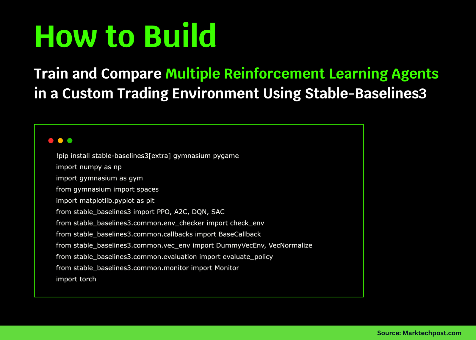
How to Build, Train, and Compare Multiple Reinforcement Learning Agents in a Custom Trading Environment Using Stable-Baselines3

In this tutorial, we explore advanced applications of Stable-Baselines3 in reinforcement learning. We design a fully functional, custom trading environment, integrate multiple algorithms such as PPO and A2C, and develop our own training callbacks for performance tracking. As we progress, we train, evaluate, and visualize agent performance to compare algorithmic efficiency, learning curves, and decision strategies, all within a streamlined workflow that runs entirely offline. Check out the FULL CODES here.

!pip install stable-baselines3[extra] gymnasium pygame
import numpy as np
import gymnasium as gym
from gymnasium import spaces
import matplotlib.pyplot as plt
from stable_baselines3 import PPO, A2C, DQN, SAC
from stable_baselines3.common.env_checker import check_env
from stable_baselines3.common.callbacks import BaseCallback
from stable_baselines3.common.vec_env import DummyVecEnv, VecNormalize
from stable_baselines3.common.evaluation import evaluate_policy
from stable_baselines3.common.monitor import Monitor
import torch


class TradingEnv(gym.Env):
   def __init__(self, max_steps=200):
       super().__init__()
       self.max_steps = max_steps
       self.action_space = spaces.Discrete(3)
       self.observation_space = spaces.Box(low=-np.inf, high=np.inf, shape=(5,), dtype=np.float32)
       self.reset()
   def reset(self, seed=None, options=None):
       super().reset(seed=seed)
       self.current_step = 0
       self.balance = 1000.0
       self.shares = 0
       self.price = 100.0
       self.price_history = [self.price]
       return self._get_obs(), {}
   def _get_obs(self):
       price_trend = np.mean(self.price_history[-5:]) if len(self.price_history) >= 5 else self.price
       return np.array([
           self.balance / 1000.0,
           self.shares / 10.0,
           self.price / 100.0,
           price_trend / 100.0,
           self.current_step / self.max_steps
       ], dtype=np.float32)
   def step(self, action):
       self.current_step += 1
       trend = 0.001 * np.sin(self.current_step / 20)
       self.price *= (1 + trend + np.random.normal(0, 0.02))
       self.price = np.clip(self.price, 50, 200)
       self.price_history.append(self.price)
       reward = 0
       if action == 1 and self.balance >= self.price:
           shares_to_buy = int(self.balance / self.price)
           cost = shares_to_buy * self.price
           self.balance -= cost
           self.shares += shares_to_buy
           reward = -0.01
       elif action == 2 and self.shares > 0:
           revenue = self.shares * self.price
           self.balance += revenue
           self.shares = 0
           reward = 0.01
       portfolio_value = self.balance + self.shares * self.price
       reward += (portfolio_value - 1000) / 1000
       terminated = self.current_step >= self.max_steps
       truncated = False
       return self._get_obs(), reward, terminated, truncated, {"portfolio": portfolio_value}
   def render(self):
       print(f"Step: {self.current_step}, Balance: ${self.balance:.2f}, Shares: {self.shares}, Price: ${self.price:.2f}")

We define our custom TradingEnv, where an agent learns to make buy, sell, or hold decisions based on simulated price movements. We define the observation and action spaces, implement the reward structure, and ensure our environment reflects a realistic market scenario with fluctuating trends and noise. Check out the FULL CODES here.

class ProgressCallback(BaseCallback):
   def __init__(self, check_freq=1000, verbose=1):
       super().__init__(verbose)
       self.check_freq = check_freq
       self.rewards = []
   def _on_step(self):
       if self.n_calls % self.check_freq == 0:
           mean_reward = np.mean([ep_info["r"] for ep_info in self.model.ep_info_buffer])
           self.rewards.append(mean_reward)
           if self.verbose:
               print(f"Steps: {self.n_calls}, Mean Reward: {mean_reward:.2f}")
       return True


print("=" * 60)
print("Setting up custom trading environment...")
env = TradingEnv()
check_env(env, warn=True)
print("✓ Environment validation passed!")
env = Monitor(env)
vec_env = DummyVecEnv([lambda: env])
vec_env = VecNormalize(vec_env, norm_obs=True, norm_reward=True)

Here, we create a ProgressCallback to monitor training progress and record mean rewards at regular intervals. We then validate our custom environment using Stable-Baselines3’s built-in checker, wrap it for monitoring and normalization, and prepare it for training across multiple algorithms. Check out the FULL CODES here.

print("\n" + "=" * 60)
print("Training multiple RL algorithms...")
algorithms = {
   "PPO": PPO("MlpPolicy", vec_env, verbose=0, learning_rate=3e-4, n_steps=2048),
   "A2C": A2C("MlpPolicy", vec_env, verbose=0, learning_rate=7e-4),
}
results = {}
for name, model in algorithms.items():
   print(f"\nTraining {name}...")
   callback = ProgressCallback(check_freq=2000, verbose=0)
   model.learn(total_timesteps=50000, callback=callback, progress_bar=True)
   results[name] = {"model": model, "rewards": callback.rewards}
   print(f"✓ {name} training complete!")


print("\n" + "=" * 60)
print("Evaluating trained models...")
eval_env = Monitor(TradingEnv())
for name, data in results.items():
   mean_reward, std_reward = evaluate_policy(data["model"], eval_env, n_eval_episodes=20, deterministic=True)
   results[name]["eval_mean"] = mean_reward
   results[name]["eval_std"] = std_reward
   print(f"{name}: Mean Reward = {mean_reward:.2f} +/- {std_reward:.2f}")

We train and evaluate two different reinforcement learning algorithms, PPO and A2C, on our trading environment. We log their performance metrics, capture mean rewards, and compare how efficiently each agent learns profitable trading strategies through consistent exploration and exploitation. Check out the FULL CODES here.

print("\n" + "=" * 60)
print("Generating visualizations...")
fig, axes = plt.subplots(2, 2, figsize=(14, 10))
ax = axes[0, 0]
for name, data in results.items():
   ax.plot(data["rewards"], label=name, linewidth=2)
ax.set_xlabel("Training Checkpoints (x1000 steps)")
ax.set_ylabel("Mean Episode Reward")
ax.set_title("Training Progress Comparison")
ax.legend()
ax.grid(True, alpha=0.3)


ax = axes[0, 1]
names = list(results.keys())
means = [results[n]["eval_mean"] for n in names]
stds = [results[n]["eval_std"] for n in names]
ax.bar(names, means, yerr=stds, capsize=10, alpha=0.7, color=['#1f77b4', '#ff7f0e'])
ax.set_ylabel("Mean Reward")
ax.set_title("Evaluation Performance (20 episodes)")
ax.grid(True, alpha=0.3, axis="y")


ax = axes[1, 0]
best_model = max(results.items(), key=lambda x: x[1]["eval_mean"])[1]["model"]
obs = eval_env.reset()[0]
portfolio_values = [1000]
for _ in range(200):
   action, _ = best_model.predict(obs, deterministic=True)
   obs, reward, done, truncated, info = eval_env.step(action)
   portfolio_values.append(info.get("portfolio", portfolio_values[-1]))
   if done:
       break
ax.plot(portfolio_values, linewidth=2, color="green")
ax.axhline(y=1000, color="red", linestyle="--", label="Initial Value")
ax.set_xlabel("Steps")
ax.set_ylabel("Portfolio Value ($)")
ax.set_title(f"Best Model ({max(results.items(), key=lambda x: x[1]['eval_mean'])[0]}) Episode")
ax.legend()
ax.grid(True, alpha=0.3)

We visualize our training results by plotting learning curves, evaluation scores, and portfolio trajectories for the best-performing model. We also analyze how the agent’s actions translate into portfolio growth, which helps us interpret model behavior and assess decision consistency during simulated trading sessions. Check out the FULL CODES here.

ax = axes[1, 1]
obs = eval_env.reset()[0]
actions = []
for _ in range(200):
   action, _ = best_model.predict(obs, deterministic=True)
   actions.append(action)
   obs, _, done, truncated, _ = eval_env.step(action)
   if done:
       break
action_names = ['Hold', 'Buy', 'Sell']
action_counts = [actions.count(i) for i in range(3)]
ax.pie(action_counts, labels=action_names, autopct="%1.1f%%", startangle=90, colors=['#ff9999', '#66b3ff', '#99ff99'])
ax.set_title("Action Distribution (Best Model)")
plt.tight_layout()
plt.savefig('sb3_advanced_results.png', dpi=150, bbox_inches="tight")
print("✓ Visualizations saved as 'sb3_advanced_results.png'")
plt.show()


print("\n" + "=" * 60)
print("Saving and loading models...")
best_name = max(results.items(), key=lambda x: x[1]["eval_mean"])[0]
best_model = results[best_name]["model"]
best_model.save(f"best_trading_model_{best_name}")
vec_env.save("vec_normalize.pkl")
loaded_model = PPO.load(f"best_trading_model_{best_name}")
print(f"✓ Best model ({best_name}) saved and loaded successfully!")
print("\n" + "=" * 60)
print("TUTORIAL COMPLETE!")
print(f"Best performing algorithm: {best_name}")
print(f"Final evaluation score: {results[best_name]['eval_mean']:.2f}")
print("=" * 60)

Finally, we visualize the action distribution of the best agent to understand its trading tendencies and save the top-performing model for reuse. We demonstrate model loading, confirm the best algorithm, and complete the tutorial with a clear summary of performance outcomes and insights gained.

In conclusion, we have created, trained, and compared multiple reinforcement learning agents in a realistic trading simulation using Stable-Baselines3. We observe how each algorithm adapts to market dynamics, visualize their learning trends, and identify the most profitable strategy. This hands-on implementation strengthens our understanding of RL pipelines and demonstrates how customizable, efficient, and scalable Stable-Baselines3 can be for complex, domain-specific tasks such as financial modeling.

Check out the FULL CODES here. Feel free to check out our GitHub Page for Tutorials, Codes and Notebooks. Also, feel free to follow us on Twitter and don’t forget to join our 100k+ ML SubReddit and Subscribe to our Newsletter. Wait! are you on telegram? now you can join us on telegram as well.

Asif Razzaq is the CEO of Marktechpost Media Inc.. As a visionary entrepreneur and engineer, Asif is committed to harnessing the potential of Artificial Intelligence for social good. His most recent endeavor is the launch of an Artificial Intelligence Media Platform, Marktechpost, which stands out for its in-depth coverage of machine learning and deep learning news that is both technically sound and easily understandable by a wide audience. The platform boasts of over 2 million monthly views, illustrating its popularity among audiences.

🙌 Follow MARKTECHPOST: Add us as a preferred source on Google.

Source_link