If you’ve ever been curious about what it takes to build a language model from scratch with JAX, this post is for you. I recently ran a workshop on this topic at Cloud Next 2025 and got some great feedback, so I thought I’d write up a guide for everyone who couldn’t make it.
In this article and code example, you’re going to build and pretrain a GPT-2 model, showing how JAX makes it straightforward to leverage the power of Google TPUs. You can run the entire project for free using the TPUs in Colab or Kaggle, and you can find the full notebook here.
This is a hands-on tutorial, so I’ll assume you’re familiar with general machine learning concepts. If JAX is new to you, the PyTorch developer’s guide to JAX fundamentals is a great place to start.
First, let’s take a quick look at the tools we’ll be using.
JAX ecosystem
Before we start building the model, let’s briefly talk about the JAX ecosystem. The JAX ecosystem takes a modular approach, with JAX core providing the core numerical processing capabilities, and a rich collection of libraries built on top to serve different application-specific needs, for example, Flax for building neural networks, Orbax for checkpointing and model persistence, and Optax for optimization (we are going to use all 3 in this article). Built-in function transformations, such as autograd, vectorization and JIT compilation, plus strong performance and easy-to-use APIs, make JAX perfect for training Large Language Models.
Getting started: Build your GPT2 model
OpenAI previously released the GPT2 model code and weights, which are good references, and there are many community efforts, such as nanoGPT, to replicate the model. Here is a high level model architecture diagram for GPT2:
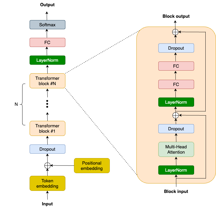
We are going to use NNX (the new Flax interface) to build the GPT2 model. For brevity, let’s focus on the transformer block, which is the key for modern large language models. The transformer block captures long-range dependencies in any sequence and builds a rich contextual understanding of it. A GPT2 transformer block consists of 2 LayerNorm layers, 1 Multi-Head Attention (MHA) layer, 2 dropout layers, 2 linear projection layers and 2 residual connections. So we first define these layers in the __init__ function of the TransformerBlock class:
class TransformerBlock(nnx.Module):
    def __init__(
        self,
        embed_dim: int,
        num_heads: int,
        ff_dim: int,
        dropout_rate: float,
        rngs: nnx.Rngs,
    ):
        self.layer_norm1 = nnx.LayerNorm(
            epsilon=1e-6, num_features=embed_dim, rngs=rngs
        )
        self.mha = nnx.MultiHeadAttention(
            num_heads=num_heads, in_features=embed_dim, rngs=rngs
        )
        self.dropout1 = nnx.Dropout(rate=dropout_rate)
        self.layer_norm2 = nnx.LayerNorm(
            epsilon=1e-6, num_features=embed_dim, rngs=rngs
        )
        self.linear1 = nnx.Linear(
            in_features=embed_dim, out_features=ff_dim, rngs=rngs
        )
        self.linear2 = nnx.Linear(
            in_features=ff_dim, out_features=embed_dim, rngs=rngs
        )
        self.dropout2 = nnx.Dropout(rate=dropout_rate)
Python
Next we assemble these layers in the __call__ function:
class TransformerBlock(nnx.Module):
    def __call__(self, inputs, training: bool = False):
        input_shape = inputs.shape
        bs, seq_len, emb_sz = input_shape

        attention_output = self.mha(
            inputs_q=self.layer_norm1(inputs),
            mask=causal_attention_mask(seq_len),
            decode=False,
        )
        x = inputs + self.dropout1(
            attention_output, deterministic=not training
        )

        # MLP
        mlp_output = self.linear1(self.layer_norm2(x))
        mlp_output = nnx.gelu(mlp_output)
        mlp_output = self.linear2(mlp_output)
        mlp_output = self.dropout2(
            mlp_output, deterministic=not training
        )

        return x + mlp_output
Python
This code should look very familiar if you have used any other ML framework, like PyTorch or TensorFlow, to train a language model. But one of the things I really like about JAX is that it has the amazing capability to automatically run the code in parallel via SPMD (Single Program Multiple Data), which is needed because we will be running the code on multiple accelerators (multiple TPU cores). Let’s see how it works.
To perform SPMD, first we need to make sure we are using TPUs. Choose the TPU runtime if you are using Colab or Kaggle (you can also use a Cloud TPU VM).
import jax
jax.devices()

# Free-tier Colab offers TPU v2:
# [TpuDevice(id=0, process_index=0, coords=(0,0,0), core_on_chip=0),
#  TpuDevice(id=1, process_index=0, coords=(0,0,0), core_on_chip=1),
#  TpuDevice(id=2, process_index=0, coords=(1,0,0), core_on_chip=0),
#  TpuDevice(id=3, process_index=0, coords=(1,0,0), core_on_chip=1),
#  TpuDevice(id=4, process_index=0, coords=(0,1,0), core_on_chip=0),
#  TpuDevice(id=5, process_index=0, coords=(0,1,0), core_on_chip=1),
#  TpuDevice(id=6, process_index=0, coords=(1,1,0), core_on_chip=0),
#  TpuDevice(id=7, process_index=0, coords=(1,1,0), core_on_chip=1)]
Python
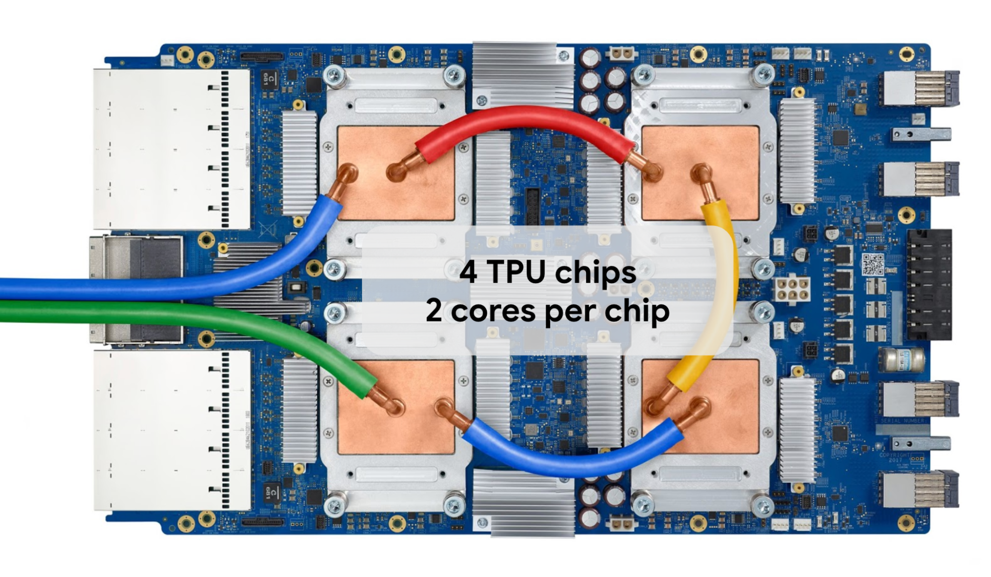
Colab and Kaggle offer a TPU v2 or v3, which has 8 separate TPU cores. Here is what a TPU v3 tray looks like:
Train your GPT2 model
To train the GPT2 model efficiently, we will run all TPU cores together via SPMD and leverage data parallelism in JAX. To achieve this, we define a hardware mesh:
mesh = jax.make_mesh((8, 1), ('batch', 'model'))Python
Think of the mesh as a 2D matrix of accelerators. In this case, we define 2 axes for the mesh – the batch axis and the model axis. So in total we have 8 by 1, which is 8 cores. These axes determine how we partition the data and the model parameters. We can change the axes later if we want to experiment with other parallelism schemes.
Now we change the __init__ function by telling JAX how we would like to partition the model parameters using the ‘model’ axis. This is done by adding nnx.with_partitioning when initializing the weight tensors: for 1D weight tensors like LayerNorm scale/bias tensors, we directly shard them along the ‘model’ axis; for 2D weight tensors like MHA and Linear kernel tensors, we shard the 2nd dimension along the model axis.
class TransformerBlock(nnx.Module):
    def __init__(
        self,
        embed_dim: int,
        num_heads: int,
        ff_dim: int,
        dropout_rate: float,
        rngs: nnx.Rngs,
    ):
        self.layer_norm1 = nnx.LayerNorm(
            epsilon=1e-6, num_features=embed_dim,rngs=rngs, rngs=rngs,
            scale_init=nnx.with_partitioning(
                nnx.initializers.ones_init(),
                ("model"),
            ),
            bias_init=nnx.with_partitioning(
                nnx.initializers.zeros_init(),
               ("model"),
            ),
        )
        self.mha = nnx.MultiHeadAttention(
            num_heads=num_heads, in_features=embed_dim,
            kernel_init=nnx.with_partitioning(
                nnx.initializers.xavier_uniform(),
               (None, "model"),
            ),
            bias_init=nnx.with_partitioning(
                nnx.initializers.zeros_init(),
               ("model"),
            ),
        )
        # Other layers in the block are omitted for brevity
Python
We need to partition other layers like this so that we can enable model tensor parallelism for the entire GPT2 model. Even though we don’t use model tensor parallelism in this tutorial, it’s still a good idea to implement this because the model size may grow and we may need to partition our model parameters in the future. Having implemented this allows us to change just one line of code and immediately run bigger models. For example,
mesh = jax.make_mesh((4, 2), ('batch', 'model'))Python
Next, we define the loss_fn and train_step functions similar to the previous blog. The train_step() function computes the gradients of the cross-entropy loss function and updates the weights via the optimizer, and it will be called in a loop to train the model. To achieve the best performance, we are JIT-compiling both functions using the @nnx.jit decorator, since they are compute intensive.
@nnx.jit
def loss_fn(model, batch):
    logits = model(batch[0])
    loss = optax.softmax_cross_entropy_with_integer_labels(
        logits=logits, labels=batch[1]
    ).mean()
    return loss, logits


@nnx.jit
def train_step(
    model: nnx.Module,
    optimizer: nnx.Optimizer,
    metrics: nnx.MultiMetric,
    batch,
):
    grad_fn = nnx.value_and_grad(loss_fn, has_aux=True)
    (loss, logits), grads = grad_fn(model, batch)
    metrics.update(loss=loss, logits=logits, lables=batch[1])
    optimizer.update(grads)
Python
For the optimizer, we are using AdamW from Optax with a cosine decay schedule. You can experiment with other optimizers or schedules in Optax as well.
schedule = optax.cosine_decay_schedule(
    init_value=init_learning_rate, decay_steps=max_steps
)
optax_chain = optax.chain(
    optax.adamw(learning_rate=schedule, weight_decay=weight_decay)
)
optimizer = nnx.Optimizer(model, optax_chain)
Python
Lastly, we create a simple training loop.
while True:
    input_batch, target_batch = get_batch("train")

    train_step(
        model,
        optimizer,
        train_metrics,
        jax.device_put(
            (input_batch, target_batch),
            NamedSharding(mesh, P("batch", None)),
        ),
    )

    step += 1
    if step > max_steps:
        break
Python
Note how we partition the input data along the batch axis using the jax.device_put function. In this case JAX will enable data parallelism and bring everything together by inserting communication collectives (AllReduce) automatically, and overlap computation and communication as much as possible. For a more in-depth discussion on parallel computation, please refer to JAX’s Introduction to parallel programming documentation.
At this point the model should be training and we can observe the training loss if Weights and Biases is used to track the run. Here is a test run for training the GPT2 124M model:
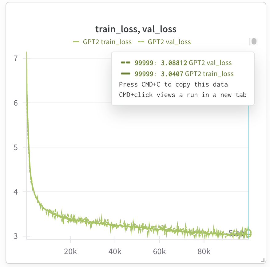
It takes ~7 hours on Kaggle TPU v3 (which we can use for 9 hours without interruption), but if we use Trillium, training time goes down to ~1.5 hours (note that Trillium has 32G HBM (High Bandwidth Memory) per chip, so we can double the batch size and halve the training steps).
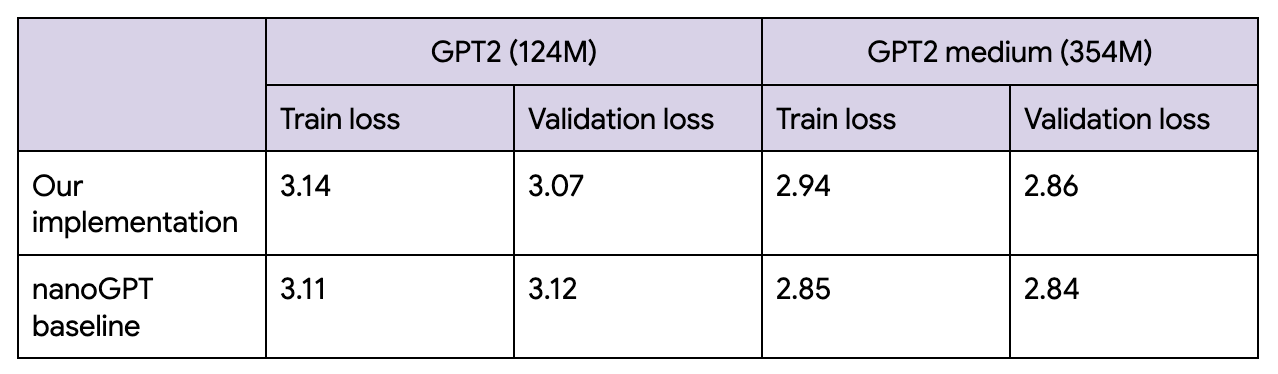
Final losses are roughly in line with nanoGPT’s, which I really enjoyed, and studied while writing this code example.
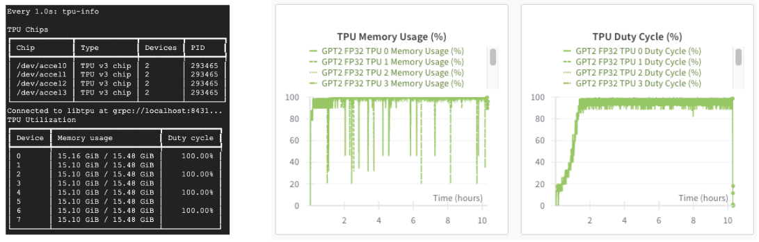
If we use Cloud TPUs, we can also monitor the TPU utilization via the ‘tpu-info’ command (part of the Cloud TPU Monitoring Debugging package) or Weights and Biases dashboard. Our TPUs are going brrr!
After the model is trained, we can save it using Orbax:
checkpointer = orbax.PyTreeCheckpointer()
train_state = nnx.pure(nnx.state(model))
checkpointer.save(checkpoint_path, train_state)
Python
Next steps: Explore advanced LLM training and scaling
That’s it. That’s pretty much all we need to train a GPT2 model. You can find additional details like data loading, hyperparameters, metrics, in the complete notebook.
Of course GPT2 is a small model today and many frontier labs are training models with hundreds of billions of parameters. But now that you have learned how to build a small language model with JAX and TPU, you are ready to dive into How to scale your model.
In addition, you can either use MaxText to train pre-built cutting edge LLMs or learn to build the latest models from scratch by referencing the JAX LLM examples or the Stanford Marin model.
I can’t wait to see the amazing models you build with JAX and TPUs!