In this article, you will learn how to turn a raw time series into a supervised learning dataset and use decision tree-based models to forecast future values.
Topics we will cover include:
- Engineering lag features and rolling statistics from a univariate series.
- Preparing a chronological train/test split and fitting a decision tree regressor.
- Evaluating with MAE and avoiding data leakage with proper feature design.
Let’s not waste any more time.

Forecasting the Future with Tree-Based Models for Time Series
Image by Editor
Introduction
Decision tree-based models in machine learning are frequently used for a wide range of predictive tasks such as classification and regression, typically on structured, tabular data. However, when combined with the right data processing and feature extraction approaches, decision trees also become a powerful predictive tool for other data formats like text, images, or time series.
This article demonstrates how decision trees can be used to perform time series forecasting. More specifically, we show how to extract significant features from raw time series — such as lagged features and rolling statistics — and leverage this structured information to perform the aforementioned predictive tasks by training decision tree-based models.
Building Decision Trees for Time Series Forecasting
In this hands-on tutorial, we will use the monthly airline passengers dataset available for free in the sktime library. This is a small univariate time series dataset containing monthly passenger numbers for an airline indexed by year-month, between 1949 and 1960.
Let’s start by loading the dataset — you may need to pip install sktime first if you haven’t used the library before:
|
import pandas as pd from sktime.datasets import load_airline
y = load_airline() y.head() |
Since this is a univariate time series, it is managed as a one-dimensional pandas Series indexed by date (month-year), rather than a two-dimensional DataFrame object.
To extract relevant features from our time series and turn it into a fully structured dataset, we define a custom function called make_lagged_df_with_rolling, which takes the raw time series as input, plus two keyword arguments: lags and roll_window, which we will explain shortly:
|
def make_lagged_df_with_rolling(series, lags=12, roll_window=3): df = pd.DataFrame({“y”: series})
for lag in range(1, lags+1): df[f“lag_{lag}”] = df[“y”].shift(lag)
df[f“roll_mean_{roll_window}”] = df[“y”].shift(1).rolling(roll_window).mean() df[f“roll_std_{roll_window}”] = df[“y”].shift(1).rolling(roll_window).std()
return df.dropna()
df_features = make_lagged_df_with_rolling(y, lags=12, roll_window=3) df_features.head() |
Time to revisit the above code and see what happened inside the function:
- We first force our univariate time series to become a pandas
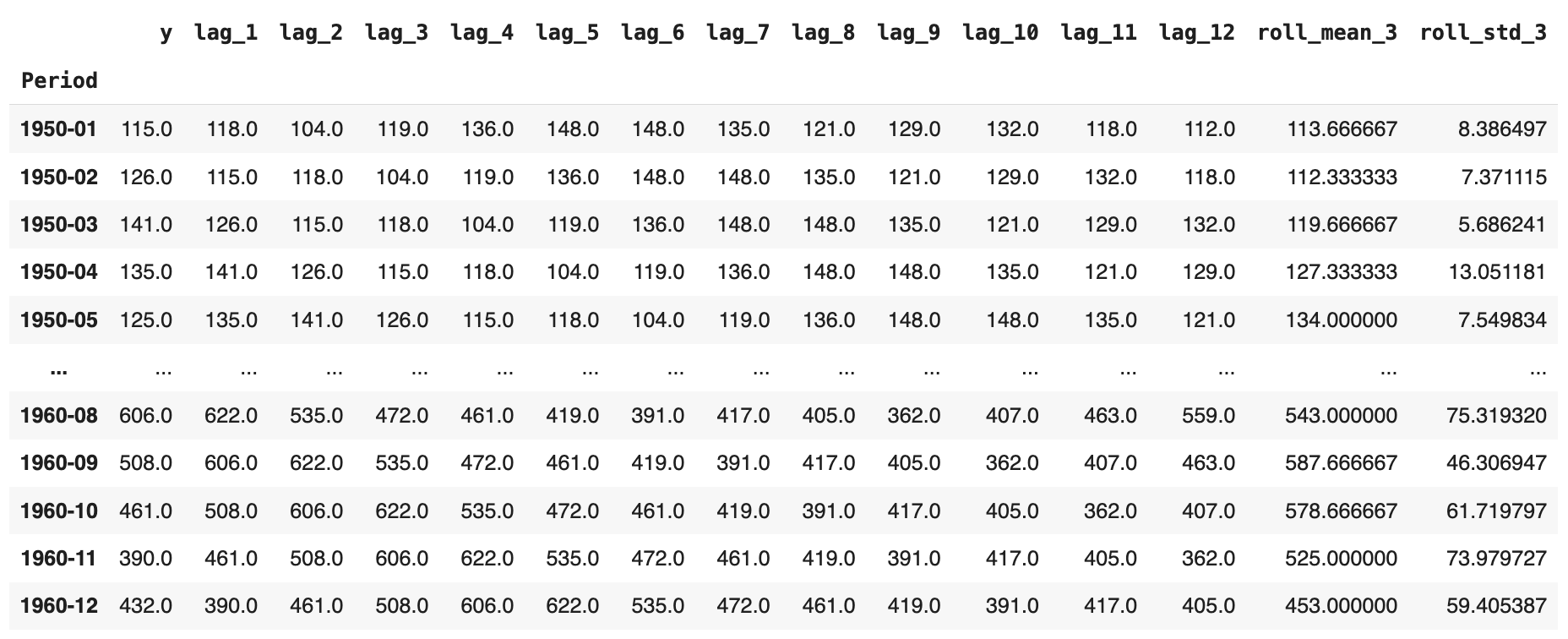
DataFrame, as we will shortly expand it with several additional features. - We incorporate lagged features; i.e., given a specific passenger value at a timestamp, we collect the previous values from preceding months. In our scenario, at time t, we include all consecutive readings from t-1 up to t-12 months earlier, as shown in the image below. For January 1950, for instance, we have both the original passenger numbers and the equivalent values for the previous 12 months added across 12 additional attributes, in reverse temporal order.
- Finally, we add two more attributes containing the rolling average and rolling standard deviation, respectively, spanning three months. That is, given a monthly reading of passenger numbers, we calculate the average or standard deviation of the latest n = 3 months excluding the current month (see the use of
.shift(1)before the.rolling()call), which prevents look-ahead leakage.
The resulting enriched dataset should look like this:
After that, training and testing the decision tree is straightforward and done as usual with scikit-learn models. The only aspect to keep in mind is: what will be our target variable to predict? Of course, we want to forecast “unknown” values of passenger numbers at a given month based on the rest of the features extracted. Therefore, the original time series variable becomes our target label. Also, make sure you choose the DecisionTreeRegressor, as we are focused on numerical predictions in this scenario, not classifications:
Partitioning the dataset into training and test, and separating the labels from predictor features:
|
train_size = int(len(df_features) * 0.8) train, test = df_features.iloc[:train_size], df_features.iloc[train_size:]
X_train, y_train = train.drop(“y”, axis=1), train[“y”] X_test, y_test = test.drop(“y”, axis=1), test[“y”] |
Training and evaluating the decision tree error (MAE):
|
from sklearn.tree import DecisionTreeRegressor from sklearn.metrics import mean_absolute_error
dt_reg = DecisionTreeRegressor(max_depth=5, random_state=42) dt_reg.fit(X_train, y_train) y_pred = dt_reg.predict(X_test)
print(“Forecasting:”) print(“MAE:”, mean_absolute_error(y_test, y_pred)) |
In one run, the resulting error was MAE ≈ 45.32. That is not bad, considering that monthly passenger numbers in the dataset are in the several hundreds; of course, there is room for improvement by using ensembles, extracting additional features, tuning hyperparameters, or exploring alternative models.
A final takeaway: unlike traditional time series forecasting methods, which predict a future or unknown value based solely on past values of the same variable, the decision tree we built predicts that value based on other features we created. In practice, it is often effective to combine both approaches with two different model types to obtain more robust predictions.
Wrapping Up
This article showed how to train decision tree models capable of dealing with time series data by extracting features from them. Starting with a raw univariate time series of monthly passenger numbers for an airline, we extracted lagged features and rolling statistics to act as predictor attributes and performed forecasting via a trained decision tree.