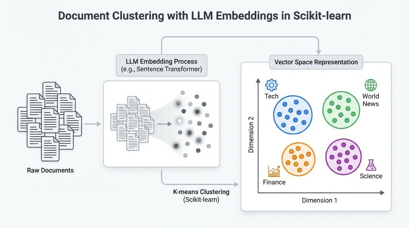
In this article, you will learn how to cluster a collection of text documents using large language model embeddings and standard clustering algorithms in scikit-learn.
Topics we will cover include:
- Why LLM-based embeddings are well suited for document clustering.
- How to generate embeddings from raw text using a pre-trained sentence transformer.
- How to apply and compare k-means and DBSCAN for clustering embedded documents.
Let’s get straight to the point.

Document Clustering with LLM Embeddings in Scikit-learn (click to enlarge)
Image by Editor
Introduction
Imagine that you suddenly obtain a large collection of unclassified documents and are tasked with grouping them by topic. There are traditional clustering methods for text, based on TF-IDF and Word2Vec, that can address this problem, but they suffer from important limitations:
- TF-IDF only counts words in a text and relies on similarity based on word frequencies, ignoring the underlying meaning. A sentence like “the tree is big” has an identical representation whether it refers to a natural tree or a decision tree classifier used in machine learning.
- Word2Vec captures relationships between individual words to form embeddings (numerical vector representations), but it does not explicitly model full context across longer text sequences.
Meanwhile, modern embeddings generated by large language models, such as sentence transformer models, are in most cases superior. They capture contextual semantics — for example, distinguishing natural trees from decision trees — and encode overall, document-level meaning. Moreover, these embeddings are produced by models pre-trained on millions of texts, meaning they already contain a substantial amount of general language knowledge.
This article follows up on a previous tutorial, where we learned how to convert raw text into large language model embeddings that can be used as features for downstream machine learning tasks. Here, we focus specifically on using embeddings from a collection of documents for clustering based on similarity, with the goal of identifying common topics among documents in the same cluster.
Step-by-Step Guide
Let’s walk through the full process using Python.
Depending on your development environment or notebook configuration, you may need to pip install some of the libraries imported below. Assuming they are already available, we start by importing the required modules and classes, including KMeans, scikit-learn’s implementation of the k-means clustering algorithm:
|
import pandas as pd import numpy as np from sentence_transformers import SentenceTransformer from sklearn.cluster import KMeans from sklearn.decomposition import PCA from sklearn.metrics import silhouette_score, adjusted_rand_score from sklearn.preprocessing import LabelEncoder import matplotlib.pyplot as plt import seaborn as sns
# Configurations for clearer visualizations sns.set_style(“whitegrid”) plt.rcParams[‘figure.figsize’] = (12, 6) |
Next, we load the dataset. We will use a BBC News dataset containing articles labeled by topic, with a public version available from a Google-hosted dataset repository:
|
url = “https://storage.googleapis.com/dataset-uploader/bbc/bbc-text.csv” df = pd.read_csv(url)
print(f“Dataset loaded: {len(df)} documents”) print(f“Categories: {df[‘category’].unique()}\n”) print(df[‘category’].value_counts()) |
Here, we only display information about the categories to get a sense of the ground-truth topics assigned to each document. The dataset contains 2,225 documents in the version used at the time of writing.
At this point, we are ready for the two main steps of the workflow: generating embeddings from raw text and clustering those embeddings.
Generating Embeddings with a Pre-Trained Model
Libraries such as sentence_transformers make it straightforward to use a pre-trained model for tasks like generating embeddings from text. The workflow consists of loading a suitable model — such as all-MiniLM-L6-v2, a lightweight model trained to produce 384-dimensional embeddings — and running inference over the dataset to convert each document into a numerical vector that captures its overall semantics.
We start by loading the model:
|
# Load embeddings model (downloaded automatically on first use) print(“Loading embeddings model…”) model = SentenceTransformer(‘all-MiniLM-L6-v2’)
# This model converts text into a 384-dimensional vector print(f“Model loaded. Embedding dimension: {model.get_sentence_embedding_dimension()}”) |
Next, we generate embeddings for all documents:
|
# Convert all documents into embedding vectors print(“Generating embeddings (this may take a few minutes)…”)
texts = df[‘text’].tolist() embeddings = model.encode( texts, show_progress_bar=True, batch_size=32 # Batch processing for efficiency )
print(f“Embeddings generated: matrix size is {embeddings.shape}”) print(f” → Each document is now represented by {embeddings.shape[1]} numeric values”) |
Recall that an embedding is a high-dimensional numerical vector. Documents that are semantically similar are expected to have embeddings that are close to each other in this vector space.
Clustering Document Embeddings with K-Means
Applying the k-means clustering algorithm with scikit-learn is straightforward. We pass in the embedding matrix and specify the number of clusters to find. While this number must be chosen in advance for k-means, we can leverage prior knowledge of the dataset’s ground-truth categories in this example. In other settings, techniques such as the elbow method can help guide this choice.
The following code applies k-means and evaluates the results using several metrics, including the Adjusted Rand Index (ARI). ARI is a permutation-invariant metric that compares the cluster assignments with the true category labels. Values closer to 1 indicate stronger agreement with the ground truth.
|
n_clusters = 5
kmeans = KMeans(n_clusters=n_clusters, random_state=42, n_init=10) kmeans_labels = kmeans.fit_predict(embeddings)
# Evaluation against ground-truth categories le = LabelEncoder() true_labels = le.fit_transform(df[‘category’])
print(” K-Means Results:”) print(f” Silhouette Score: {silhouette_score(embeddings, kmeans_labels):.3f}”) print(f” Adjusted Rand Index: {adjusted_rand_score(true_labels, kmeans_labels):.3f}”) print(f” Distribution: {pd.Series(kmeans_labels).value_counts().sort_index().tolist()}”) |
Example output:
|
K–Means Results: Silhouette Score: 0.066 Adjusted Rand Index: 0.899 Distribution: [376, 414, 517, 497, 421] |
Clustering Document Embeddings with DBSCAN
As an alternative, we can apply DBSCAN, a density-based clustering algorithm that automatically infers the number of clusters based on point density. Instead of specifying the number of clusters, DBSCAN requires parameters such as eps (the neighborhood radius) and min_samples:
|
from sklearn.cluster import DBSCAN
# DBSCAN often works better with cosine distance for text embeddings dbscan = DBSCAN(eps=0.5, min_samples=5, metric=‘cosine’) dbscan_labels = dbscan.fit_predict(embeddings)
# Count clusters (-1 indicates noise points) n_clusters_found = len(set(dbscan_labels)) – (1 if –1 in dbscan_labels else 0) n_noise = list(dbscan_labels).count(–1)
print(“\nDBSCAN Results:”) print(f” Clusters found: {n_clusters_found}”) print(f” Noise documents: {n_noise}”) print(f” Silhouette Score: {silhouette_score(embeddings[dbscan_labels != -1], dbscan_labels[dbscan_labels != -1]):.3f}”) print(f” Adjusted Rand Index: {adjusted_rand_score(true_labels, dbscan_labels):.3f}”) print(f” Distribution: {pd.Series(dbscan_labels).value_counts().sort_index().to_dict()}”) |
DBSCAN is highly sensitive to its hyperparameters, so achieving good results often requires careful tuning using systematic search strategies.
Once reasonable parameters have been identified, it can be informative to visually compare the clustering results. The following code projects the embeddings into two dimensions using principal component analysis (PCA) and plots the true categories alongside the k-means and DBSCAN cluster assignments:
|
1 2 3 4 5 6 7 8 9 10 11 12 13 14 15 16 17 18 19 20 21 22 23 24 25 26 27 28 29 30 31 32 33 34 35 36 37 38 39 40 41 42 43 44 45 46 47 48 49 50 51 52 53 |
# Reduce embeddings to 2D for visualization pca = PCA(n_components=2, random_state=42) embeddings_2d = pca.fit_transform(embeddings)
# Create comparative visualization fig, axes = plt.subplots(1, 3, figsize=(18, 5))
# Plot 1: True categories category_colors = {cat: i for i, cat in enumerate(df[‘category’].unique())} color_map = df[‘category’].map(category_colors)
axes[0].scatter( embeddings_2d[:, 0], embeddings_2d[:, 1], c=color_map, cmap=‘Set2’, alpha=0.6, s=30 ) axes[0].set_title(‘True Categories’, fontsize=12, fontweight=‘bold’) axes[0].set_xlabel(‘PC1’) axes[0].set_ylabel(‘PC2’)
# Plot 2: K-Means scatter2 = axes[1].scatter( embeddings_2d[:, 0], embeddings_2d[:, 1], c=kmeans_labels, cmap=‘viridis’, alpha=0.6, s=30 ) axes[1].set_title(f‘K-Means (k={n_clusters})’, fontsize=12, fontweight=‘bold’) axes[1].set_xlabel(‘PC1’) axes[1].set_ylabel(‘PC2’) plt.colorbar(scatter2, ax=axes[1])
# Plot 3: DBSCAN scatter3 = axes[2].scatter( embeddings_2d[:, 0], embeddings_2d[:, 1], c=dbscan_labels, cmap=‘plasma’, alpha=0.6, s=30 ) axes[2].set_title(f‘DBSCAN ({n_clusters_found} clusters + noise)’, fontsize=12, fontweight=‘bold’) axes[2].set_xlabel(‘PC1’) axes[2].set_ylabel(‘PC2’) plt.colorbar(scatter3, ax=axes[2])
plt.tight_layout() plt.show() |
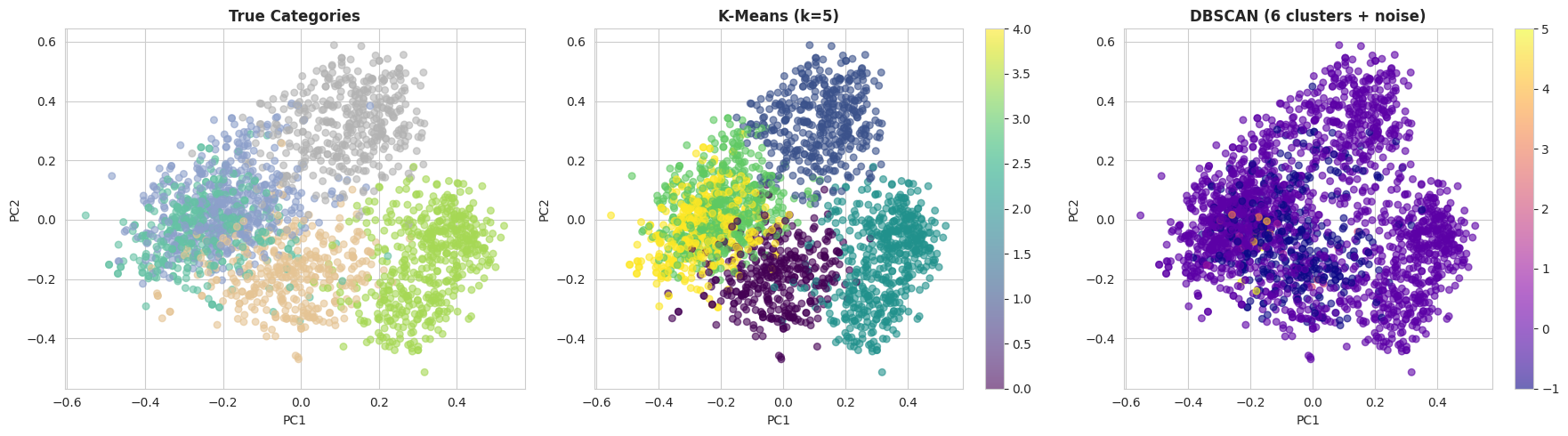
With the default DBSCAN settings, k-means typically performs much better on this dataset. There are two main reasons for this:
- DBSCAN suffers from the curse of dimensionality, and 384-dimensional embeddings can be challenging for density-based methods.
- K-means performs well when clusters are relatively well separated, which is the case for the BBC News dataset due to the clear topical structure of the documents.
Wrapping Up
In this article, we demonstrated how to cluster a collection of text documents using embedding representations generated by pre-trained large language models. After transforming raw text into numerical vectors, we applied traditional clustering techniques — k-means and DBSCAN — to group semantically similar documents and evaluate their performance against known topic labels.