In this article, you will learn how bagging, boosting, and stacking work, when to use each, and how to apply them with practical Python examples.
Topics we will cover include:
- Core ideas behind bagging, boosting, and stacking
- Step-by-step workflows and advantages of each method
- Concise, working code samples using scikit-learn
Let’s not waste any more time.
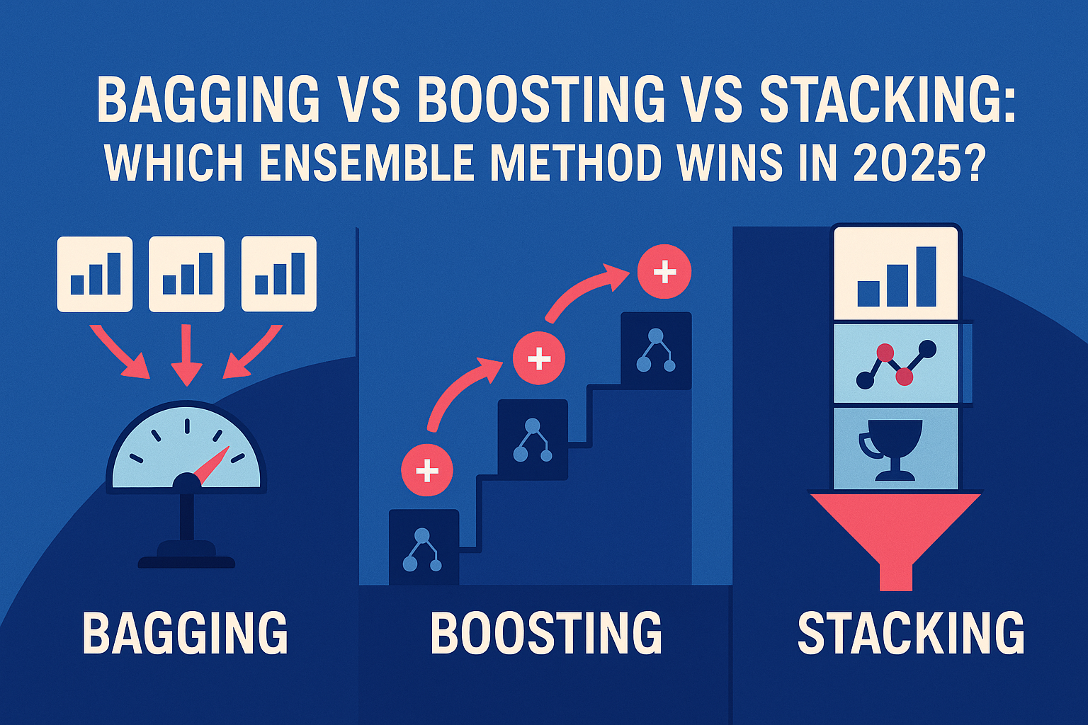
Bagging vs Boosting vs Stacking: Which Ensemble Method Wins in 2025?
Image by Editor | ChatGPT
Introduction
In machine learning, no single model is perfect. That is why data scientists use ensemble methods, which are techniques that combine multiple models to make more accurate predictions. Among the most popular are bagging, boosting, and stacking. Each works differently: Bagging reduces errors by averaging, Boosting improves results step by step, and Stacking blends different models.
In 2025, these methods are more important than ever. They power systems from recommendations to fraud detection. In this article, we will see how bagging, boosting, and stacking compare.
What Is Bagging?
Bagging, short for bootstrap aggregating, is an ensemble learning method that trains multiple models on different random subsets of the data (with replacement) and then combines their predictions.
How it works:
- Bootstrap sampling: Multiple datasets are created by sampling the training data with replacement. Each dataset is slightly different but contains roughly the same number of examples as the original dataset.
- Model training: A separate model is trained independently on each bootstrap sample.
- Aggregation: Predictions from all models are combined—by majority vote for classification or by averaging for regression.
Advantages:
- Reduces variance: By averaging many unstable models, bagging smooths out fluctuations and reduces overfitting
- Parallel training: Since models are trained independently, bagging scales well across multiple CPUs or machines
Bagging Code Example
This code trains both a bagging classifier with decision trees and a random forest classifier.
|
1 2 3 4 5 6 7 8 9 10 11 12 13 14 15 16 17 18 19 20 21 22 23 24 25 26 27 28 29 30 31 32 33 34 |
from sklearn.datasets import load_iris from sklearn.model_selection import train_test_split, cross_val_score from sklearn.metrics import accuracy_score from sklearn.tree import DecisionTreeClassifier from sklearn.ensemble import BaggingClassifier, RandomForestClassifier
# Loading data X, y = load_iris(return_X_y=True) Xtr, Xte, ytr, yte = train_test_split(X, y, test_size=0.25, random_state=42, stratify=y)
# Bagging with decision trees bag = BaggingClassifier( estimator=DecisionTreeClassifier(random_state=42), n_estimators=200, max_samples=0.8, bootstrap=True, random_state=42, n_jobs=–1 )
# Random forest rf = RandomForestClassifier( n_estimators=300, max_features=“sqrt”, random_state=42, n_jobs=–1 )
for name, model in [(“Bagging”, bag), (“RandomForest”, rf)]: cv = cross_val_score(model, X, y, cv=5, scoring=“accuracy”, n_jobs=–1) print(f“{name} CV accuracy: {cv.mean():.4f} ± {cv.std():.4f}”) model.fit(Xtr, ytr) pred = model.predict(Xte) print(f“{name} Test accuracy: {accuracy_score(yte, pred):.4f}\n”) |
Output:
|
Bagging CV accuracy: 0.9667 ± 0.0211 Bagging Test accuracy: 0.9474
RandomForest CV accuracy: 0.9667 ± 0.0211 RandomForest Test accuracy: 0.8947 |
On the iris dataset, vanilla bagging and random forests show identical mean CV accuracy (0.9667 ± 0.0211), but their single held-out test scores diverge (0.9474 vs. 0.8947). That gap is plausible on a tiny test split: random forests inject extra randomness via feature subsampling (max_features="sqrt"), which can slightly hurt when only a few strong features dominate, as in iris. In general, bagging stabilizes high-variance base learners by averaging, while random forests usually match or exceed plain bagging once trees are deep enough and there are many weakly informative features to de-correlate. With small data and minimal tuning, expect more split-to-split variability; with larger tabular datasets and tuned hyperparameters, random forests typically pull ahead due to reduced tree correlation without much bias penalty.
What Is Boosting?
Boosting is an ensemble learning technique that combines multiple weak learners (usually decision trees) to form a strong predictive model. The main idea is that instead of training one complex model, we train a sequence of weak models where each new model tries to correct the mistakes made by the previous ones.
How it works:
- Sequential training: Models are built one after another, each learning from the errors of the previous model
- Weight adjustment: Misclassified samples are given higher importance so later models focus more on difficult cases
- Model combination: All weak learners are combined using weighted voting (classification) or averaging (regression) to form a strong final model
Advantages:
- Reduces bias: By sequentially correcting errors, boosting lowers systematic bias and improves overall model accuracy
- Strong predictive power: Boosting often outperforms other ensemble methods, especially on structured/tabular datasets
// Boosting Code Example
This code applies AdaBoost with shallow decision trees and gradient boosting on the iris dataset.
|
1 2 3 4 5 6 7 8 9 10 11 12 13 14 15 16 17 18 19 20 21 22 23 24 25 26 27 28 29 30 31 32 |
from sklearn.datasets import load_iris from sklearn.model_selection import train_test_split, cross_val_score from sklearn.metrics import accuracy_score from sklearn.ensemble import AdaBoostClassifier, GradientBoostingClassifier from sklearn.tree import DecisionTreeClassifier
# Loading data X, y = load_iris(return_X_y=True) Xtr, Xte, ytr, yte = train_test_split(X, y, test_size=0.25, random_state=7, stratify=y)
# AdaBoost with shallow trees ada = AdaBoostClassifier( estimator=DecisionTreeClassifier(max_depth=2, random_state=7), n_estimators=200, learning_rate=0.5, random_state=7 )
# Gradient boosting gbrt = GradientBoostingClassifier( n_estimators=200, learning_rate=0.05, max_depth=3, random_state=7 )
for name, model in [(“AdaBoost”, ada), (“GradientBoosting”, gbrt)]: cv = cross_val_score(model, X, y, cv=5, scoring=“accuracy”, n_jobs=–1) print(f“{name} CV accuracy: {cv.mean():.4f} ± {cv.std():.4f}”) model.fit(Xtr, ytr) pred = model.predict(Xte) print(f“{name} Test accuracy: {accuracy_score(yte, pred):.4f}\n”) |
Output:
|
AdaBoost CV accuracy: 0.9600 ± 0.0327 AdaBoost Test accuracy: 0.9737
GradientBoosting CV accuracy: 0.9600 ± 0.0327 GradientBoosting Test accuracy: 0.9737 |
Both AdaBoost and gradient boosting achieve the same mean CV (0.9600 ± 0.0327) and the same test accuracy (0.9737), consistent with boosting’s bias-reduction via sequential error-correction. AdaBoost with shallow trees can excel on clean, well-separated classes like iris because re-weighting quickly focuses on the few boundary points. Gradient boosting reaches similar performance with a smaller learning rate and more estimators, trading speed for smoother fits. Broadly, boosting often wins on structured/tabular data when signal is subtle or interactions matter; however, it’s more sensitive to label noise and requires careful control of learning rate, depth, and number of trees to avoid overfitting.
What Is Stacking?
Stacking (short for stacked generalization) is an ensemble learning technique that combines predictions from multiple models (base learners) using another model (meta-learner) to make the final prediction. It leverages the strengths of different algorithms to achieve better overall performance.
How it works:
- Train base models: Several different models (e.g. decision trees, logistic regression, neural networks, etc.) are trained on the same dataset.
- Generate meta-features: The predictions of these base models are collected (instead of their raw inputs). These predictions form a new dataset.
- Train a meta-model: A new model (called a meta-learner or level-1 model) is trained on these predictions. Its job is to learn how to best combine the outputs of the base models to make the final prediction.
Advantages:
- Model diversity: Can leverage the strengths of completely different algorithms
- Highly flexible: Works with linear models, trees, neural networks, etc
Stacking Code Example
This code builds a stacking classifier using random forest, gradient boosting, and support vector machine as base learners, with logistic regression as the meta-model, and measures its performance on the iris dataset.
|
1 2 3 4 5 6 7 8 9 10 11 12 13 14 15 16 17 18 19 20 21 22 23 24 25 26 27 28 29 30 31 32 33 34 35 |
from sklearn.datasets import load_iris from sklearn.model_selection import train_test_split, cross_val_score from sklearn.metrics import accuracy_score, classification_report from sklearn.linear_model import LogisticRegression from sklearn.svm import SVC from sklearn.ensemble import RandomForestClassifier, GradientBoostingClassifier, StackingClassifier
# Loading data X, y = load_iris(return_X_y=True) Xtr, Xte, ytr, yte = train_test_split(X, y, test_size=0.25, random_state=13, stratify=y)
# Base models (level-0) base_models = [ (“rf”, RandomForestClassifier(n_estimators=200, random_state=13)), (“gb”, GradientBoostingClassifier(n_estimators=200, random_state=13)), (“svm”, SVC(kernel=“rbf”, C=1.0, probability=True, random_state=13)) ]
# Meta-model (level-1) meta = LogisticRegression(max_iter=1000, multi_class=“auto”, solver=“lbfgs”)
# Stacking classifier stack = StackingClassifier( estimators=base_models, final_estimator=meta, cv=5, # out-of-fold predictions for the meta-learner n_jobs=–1 )
cv = cross_val_score(stack, X, y, cv=5, scoring=“accuracy”, n_jobs=–1) print(f“Stacking CV accuracy: {cv.mean():.4f} ± {cv.std():.4f}”) stack.fit(Xtr, ytr) pred = stack.predict(Xte) print(f“Stacking Test accuracy: {accuracy_score(yte, pred):.4f}”) print(“\nClassification report:\n”, classification_report(yte, pred)) |
Output:
|
Stacking Test accuracy: 0.9737
Classification report: precision recall f1–score support
0 1.00 1.00 1.00 13 1 1.00 0.92 0.96 12 2 0.93 1.00 0.96 13
accuracy 0.97 38 macro avg 0.98 0.97 0.97 38 weighted avg 0.98 0.97 0.97 38 |
The stacked model posts a 0.9737 test accuracy and balanced class metrics (macro F1 ≈ 0.97), indicating the meta-learner successfully combined partially complementary errors from RF, GB, and SVM. Using out-of-fold predictions (cv=5) for the meta-features is crucial, as it limits leakage and keeps the level-1 training realistic. On a tiny dataset, stacking’s gains over the best single base learner are necessarily modest because base models already perform near-ceiling and are somewhat correlated. In larger, messier problems where models capture different inductive biases (e.g. linear vs. tree vs. kernel), stacking tends to deliver more consistent improvements.
Key Takeaways
Given the tiny sample and single splits here, we cannot generalize from these point estimates. Still, the patterns align with common experience:
- Bagging/random forests shine when variance is the main enemy and many moderately informative features exist
- Boosting often edges out others on tabular data by reducing bias and modeling interactions
- Stacking helps when you can curate diverse base learners and have enough data to train a reliable meta-model.
In the wild, expect random forests to be strong, robust baselines that are quick to train and tune, boosting to push the frontier with careful regularization (smaller learning rates, early stopping), and stacking to add incremental gains when base models make different mistakes.
As far as caveats to keep watch for, and some practical guidance to take with you, every situation is different: class imbalance, noise, feature count, and compute budgets all shift the trade-offs.
- On small datasets, simpler ensembles (RF, shallow boosting) with conservative hyperparameters and repeated CV are safer than complex stacks
- As data grows and heterogeneity increases, consider boosting first for accuracy, then layering stacking if your base models are truly diverse
- Always validate across multiple random seeds/splits and use calibration/feature importance or SHAP checks to ensure the extra accuracy isn’t coming at the cost of brittleness
We summarize these 3 ensemble techniques in the table below.
| Feature | Bagging | Boosting | Stacking |
|---|---|---|---|
| Training Style | Parallel (independent) | Sequential (focus on mistakes) | Hierarchical (multi-level) |
| Base Learners | Usually same type | Usually same type | Different models |
| Goal | Reduce variance | Reduce bias & variance | Exploit model diversity |
| Combination | Majority vote / averaging | Weighted voting | Meta-model learns combination |
| Example Algorithms | Random Forest | AdaBoost, XGBoost, LightGBM | Stacking classifier |
| Risk | High bias remains | Sensitive to noise | Risk of overfitting |