In this article, you will learn seven practical ways to turn generic LLM embeddings into task-specific, high-signal features that boost downstream model performance.
Topics we will cover include:
- Building interpretable similarity features with concept anchors
- Reducing, normalizing, and whitening embeddings to cut noise
- Creating interaction, clustering, and synthesized features
Alright — on we go.
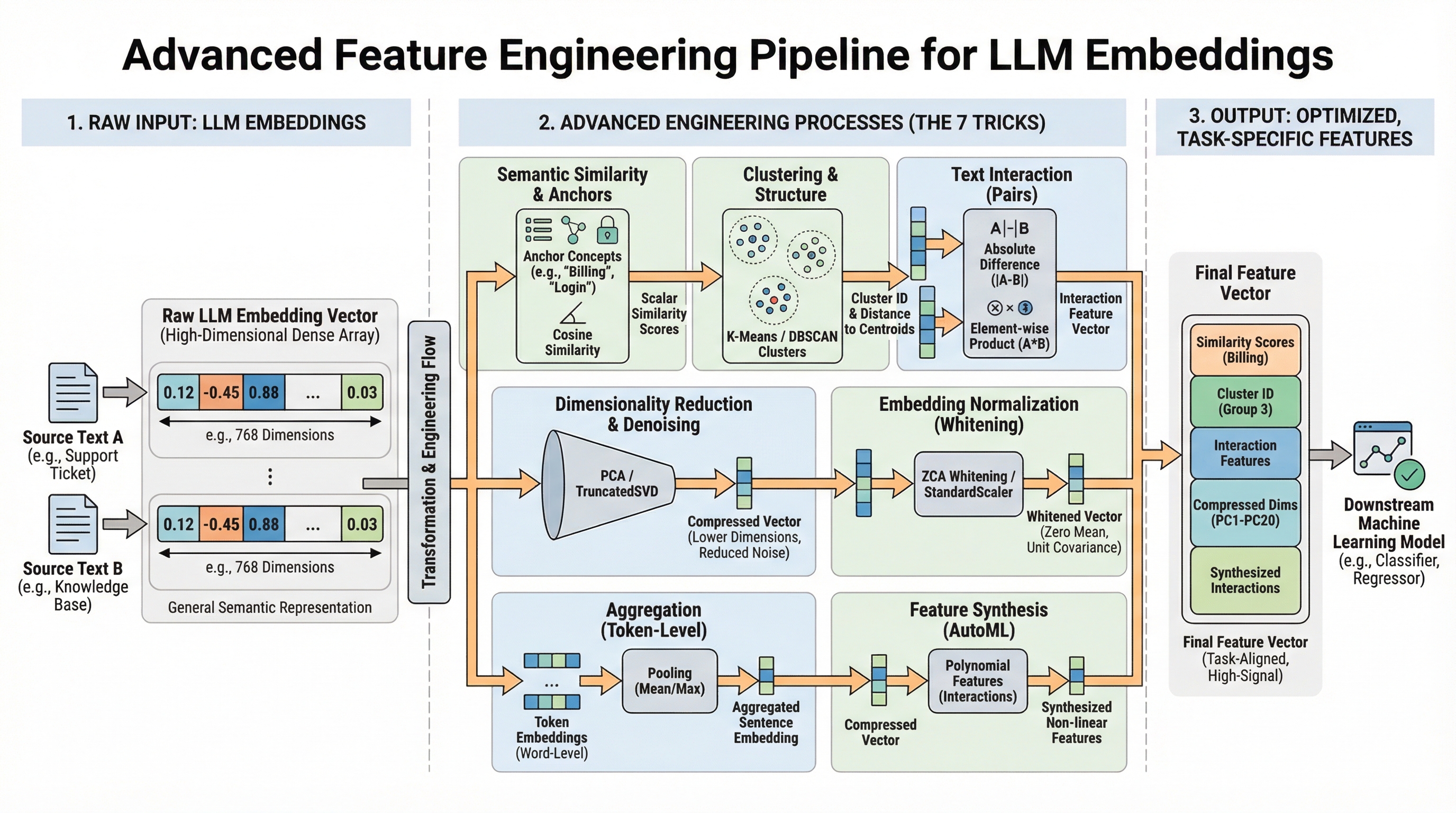
7 Advanced Feature Engineering Tricks Using LLM Embeddings
Image by Editor
The Embedding Gap
You have mastered model.encode(text) to turn words into numbers. Now what? This article moves beyond basic embedding extraction to explore seven advanced, practical techniques for transforming raw large language model (LLM) embeddings into powerful, task-specific features for your machine learning models. Using scikit-learn, sentence-transformers, and other standard libraries, we’ll translate theory into actionable code.
Modern LLMs like those provided by the sentence-transformers library generate rich, complex vector representations (embeddings) that capture semantic meaning. While using these embeddings directly can increase model performance, there’s often a gap between the general semantic knowledge in a basic embedding and the specific signal needed for your unique prediction task.
This is where advanced feature engineering comes in. By creatively processing, comparing, and decomposing these fundamental embeddings, we can extract more specific information, reduce noise, and provide our downstream models (classifiers, regressors, etc.) with features that are far more relevant. The following seven tricks are designed to close that gap.
1. Semantic Similarity as a Feature
Instead of treating an embedding as a single monolithic feature vector, calculate its similarity to key concept embeddings important to your problem. This yields understandable, scalar features.
For example, a support-ticket urgency model needs to understand whether a ticket is about “billing,” “login failure,” or a “feature request.” Raw embeddings contain this information, but a simple model cannot access it directly.
The solution is to create concept-anchor embeddings for key terms or phrases. For each text, compute the embedding’s cosine similarity to each anchor.
First you need to install sentence_transformers, sklearn, and numpy with pip. The command is the same on Windows and Linux:
|
pip install sentence_transformers sklearn numpy |
|
from sentence_transformers import SentenceTransformer from sklearn.metrics.pairwise import cosine_similarity import numpy as np
# Initialize model and encode anchors model = SentenceTransformer(‘all-MiniLM-L6-v2’) anchors = [“billing issue”, “login problem”, “feature request”] anchor_embeddings = model.encode(anchors)
# Encode a new ticket new_ticket = [“I can’t access my account, it says password invalid.”] ticket_embedding = model.encode(new_ticket)
# Calculate similarity features similarity_features = cosine_similarity(ticket_embedding, anchor_embeddings) print(similarity_features) # e.g., [[0.1, 0.85, 0.3]] -> high similarity to “login problem” |
This works because it quantifies relevance, providing the model with focused, human-interpretable signals about content themes.
Choose anchors carefully. They can be derived from domain expertise or via clustering (see Cluster Labels & Distances as Features).
2. Dimensionality Reduction and Denoising
LLM embeddings are high-dimensional (e.g., 384 or 768). Reducing dimensions can remove noise, cut computational cost, and sometimes reveal more accurate patterns.
The “curse of dimensionality” means some models (like Random Forests) may perform poorly when many dimensions are uninformative.
The solution is to use scikit-learn’s decomposition techniques to project embeddings into a lower-dimensional space.
First define your text dataset:
|
text_dataset = [ “I was charged twice for my subscription”, “Cannot reset my password”, “Would love to see dark mode added”, “My invoice shows the wrong amount”, “Login keeps failing with error 401”, “Please add export to PDF feature”, ] |
|
1 2 3 4 5 6 7 8 9 10 11 12 13 14 15 16 17 18 19 |
from sklearn.decomposition import PCA, TruncatedSVD from sklearn.manifold import TSNE # For visualization, not typically for feature engineering
# Assume ’embeddings’ is a numpy array of shape (n_samples, 384) embeddings = np.array([model.encode(text) for text in text_dataset])
# Method 1: PCA – for linear relationships # n_components must be <= min(n_samples, n_features) n_components = min(50, len(text_dataset)) pca = PCA(n_components=n_components) reduced_pca = pca.fit_transform(embeddings)
# Method 2: TruncatedSVD – similar, works on matrices from TF-IDF as well svd = TruncatedSVD(n_components=n_components) reduced_svd = svd.fit_transform(embeddings)
print(f“Original shape: {embeddings.shape}”) print(f“Reduced shape: {reduced_pca.shape}”) print(f“PCA retains {sum(pca.explained_variance_ratio_):.2%} of variance.”) |
The code above works because PCA finds axes of maximum variance, often capturing the most significant semantic information in fewer, uncorrelated dimensions.
|
Original shape: (6, 384) Reduced shape: (6, 6) PCA retains 100.00% of variance |
Note that dimensionality reduction is lossy. Always test whether reduced features maintain or improve model performance. PCA is linear; for nonlinear relationships, consider UMAP (but be mindful of its sensitivity to hyperparameters).
3. Cluster Labels and Distances as Features
Use unsupervised clustering on your collection embeddings to discover natural thematic groups. Use cluster assignments and distances to cluster centroids as new categorical and continuous features.
The problem: your data may have unknown or emerging categories not captured by predefined anchors (remember the semantic similarity trick). Clustering all document embeddings and then using the results as features addresses this.
|
1 2 3 4 5 6 7 8 9 10 11 12 13 14 15 16 17 18 19 20 |
from sklearn.cluster import KMeans, DBSCAN from sklearn.preprocessing import LabelEncoder
# Cluster the embeddings # n_clusters must be <= n_samples n_clusters = min(10, len(text_dataset)) kmeans = KMeans(n_clusters=n_clusters, random_state=42) cluster_labels = kmeans.fit_predict(embeddings)
# Feature 1: Cluster assignment (encode if your model needs numeric) encoder = LabelEncoder() cluster_id_feature = encoder.fit_transform(cluster_labels)
# Feature 2: Distance to each cluster centroid distances_to_centroids = kmeans.transform(embeddings) # Shape: (n_samples, n_clusters) # ‘distances_to_centroids’ now has up to n_clusters new continuous features per sample
# Combine with original embeddings or use alone enhanced_features = np.hstack([embeddings, distances_to_centroids]) |
This works because it provides the model with structural knowledge about the data’s natural grouping, which can be highly informative for tasks like classification or anomaly detection.
Note: we’re using n_clusters = min(10, len(text_dataset)) because we don’t have much data. Choosing the number of clusters (k) is critical—use the elbow method or domain knowledge. DBSCAN is an alternative for density-based clustering that does not require specifying k.
4. Text Difference Embeddings
For tasks involving pairs of texts (for example, duplicate-question detection and semantic search relevance), the interaction between embeddings is more important than the embeddings in isolation.
Simply concatenating two embeddings doesn’t explicitly model their relationship. A better approach is to create features that encode the difference and element-wise product between embeddings.
|
# For pairs of texts (e.g., query and document, ticket1 and ticket2) texts1 = [“I can’t log in to my account”] texts2 = [“Login keeps failing with error 401”]
embeddings1 = model.encode(texts1) embeddings2 = model.encode(texts2)
# Basic concatenation (baseline) concatenated = np.hstack([embeddings1, embeddings2])
# Advanced interaction features absolute_diff = np.abs(embeddings1 – embeddings2) # Captures magnitude of disagreement elementwise_product = embeddings1 * embeddings2 # Captures alignment (like a dot product per dimension)
# Combine all for a rich feature set interaction_features = np.hstack([embeddings1, embeddings2, absolute_diff, elementwise_product]) |
Why does this work? The difference vector highlights where semantic meanings diverge. The product vector increases where they agree. This design is influenced by successful neural network architectures like Siamese Networks used in similarity learning.
This approach roughly quadruples the feature dimension. Apply dimensionality reduction (as above) and regularization to control size and noise.
5. Embedding Whitening Normalization
If the directions of maximum variance in your dataset do not align with the most important semantic axes for your task, whitening can help. Whitening rescales and rotates embeddings to have zero mean and unit covariance, which can improve performance in similarity and retrieval tasks.
The problem is the natural directional dependence of embedding spaces (where some directions have more variance than others), which can skew distance calculations.
The solution is to apply ZCA whitening (or PCA whitening) using scikit-learn.
|
from sklearn.decomposition import PCA from sklearn.preprocessing import StandardScaler
# 1. Center the data (zero mean) scaler = StandardScaler(with_std=False) # We don’t scale std yet embeddings_centered = scaler.fit_transform(embeddings)
# 2. Apply PCA with whitening pca = PCA(whiten=True, n_components=None) # Keep all components embeddings_whitened = pca.fit_transform(embeddings_centered) |
Now cosine similarity on whitened embeddings is equivalent to correlation.
Why it works: Whitening equalizes the importance of all dimensions, preventing a few high-variance directions from dominating similarity measures. It’s a standard step in state-of-the-art semantic search pipelines like the one described in the Sentence-BERT paper.
Train the whitening transform on a representative sample. Use the same scaler and PCA objects to transform new inference data.
6. Sentence-Level vs. Word-Level Embedding Aggregation
LLMs can embed words, sentences, or paragraphs. For longer documents, strategically aggregating word-level embeddings can capture information that a single document-level embedding might miss. The problem is that a single sentence embedding for a long, multi-topic document can lose fine-grained information.
To address this, use a token-embedding model (e.g., all-MiniLM-L6-v2 in word-piece mode or bert-base-uncased from Transformers), then pool key tokens.
|
1 2 3 4 5 6 7 8 9 10 11 12 13 14 15 16 17 18 19 20 21 22 23 24 25 26 27 28 29 30 31 |
from transformers import AutoTokenizer, AutoModel import torch import numpy as np
# Load a model that provides token embeddings model_name = “bert-base-uncased” tokenizer = AutoTokenizer.from_pretrained(model_name) model = AutoModel.from_pretrained(model_name)
def get_pooled_embeddings(text, pooling_strategy=“mean”): inputs = tokenizer(text, return_tensors=“pt”, truncation=True, padding=True) with torch.no_grad(): outputs = model(**inputs) token_embeddings = outputs.last_hidden_state # Shape: (batch, seq_len, hidden_dim) attention_mask = inputs[“attention_mask”].unsqueeze(–1) # (batch, seq_len, 1)
if pooling_strategy == “mean”: # Masked mean to ignore padding tokens masked = token_embeddings * attention_mask summed = masked.sum(dim=1) counts = attention_mask.sum(dim=1).clamp(min=1) return (summed / counts).squeeze(0).numpy() elif pooling_strategy == “max”: # Very negative number for masked positions masked = token_embeddings.masked_fill(attention_mask == 0, –1e9) return masked.max(dim=1).values.squeeze(0).numpy() elif pooling_strategy == “cls”: return token_embeddings[:, 0, :].squeeze(0).numpy()
# Example: Get mean of non-padding token embeddings doc_embedding = get_pooled_embeddings(“A long document about several topics.”) |
Why it works: Mean pooling averages out noise, while max pooling highlights the most salient features. For tasks where specific keywords are critical (e.g., sentiment from “amazing” vs. “terrible”), this can be more effective than standard sentence embeddings.
Note that this can be computationally heavier than sentence-transformers. It also requires careful handling of padding and attention masks. The [CLS] token embedding is often fine-tuned for specific tasks but may be less general as a feature.
7. Embeddings as Input for Feature Synthesis (AutoML)
Let automated feature engineering tools treat your embeddings as raw input to discover complex, non-linear interactions you might not consider manually. Manually engineering interactions between hundreds of embedding dimensions is impractical.
One practical approach is to use scikit-learn’s PolynomialFeatures on reduced-dimension embeddings.
|
from sklearn.preprocessing import PolynomialFeatures from sklearn.decomposition import PCA
# Start with reduced embeddings to avoid explosion # n_components must be <= min(n_samples, n_features) n_components_poly = min(20, len(text_dataset)) pca = PCA(n_components=n_components_poly) embeddings_reduced = pca.fit_transform(embeddings)
# Generate polynomial and interaction features up to degree 2 poly = PolynomialFeatures(degree=2, interaction_only=False, include_bias=False) synthesized_features = poly.fit_transform(embeddings_reduced)
print(f“Reduced dimensions: {embeddings_reduced.shape[1]}”) print(f“Synthesized features: {synthesized_features.shape[1]}”) # n + n*(n+1)/2 features |
This code automatically creates features representing meaningful interactions between different semantic concepts captured by the principal components of your embeddings.
Because this can lead to feature explosion and overfitting, always use strong regularization (L1/L2) and rigorous validation. Apply after significant dimensionality reduction.
Conclusion
In this article you have learned that advanced feature engineering with LLM embeddings is a structured, iterative process of:
- Understanding your problem’s semantic needs
- Transforming raw embeddings into targeted signals (similarity, clusters, differences)
- Optimizing the representation (normalization, reduction)
- Synthesizing new interactions cautiously
Start by integrating one or two of these tricks into your existing pipeline. For example, combine Trick 1 (Semantic Similarity) with Trick 2 (Dimensionality Reduction) to create a powerful, interpretable feature set. Monitor validation performance carefully to see what works for your specific domain and data.
The goal is to move from seeing an LLM embedding as a black-box vector to treating it as a rich, structured semantic foundation from which you can sculpt precise features that give your models a decisive edge.