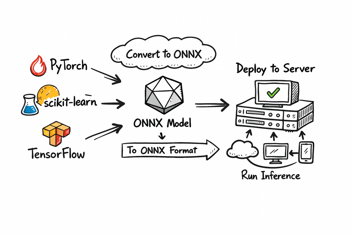
In this article, you will learn how to export models from PyTorch, scikit-learn, and TensorFlow/Keras to ONNX and compare PyTorch vs. ONNX Runtime inference on CPU for accuracy and speed.
Topics we will cover include:
- Fine-tuning a ResNet-18 on CIFAR-10 and exporting it to ONNX.
- Verifying numerical parity and benchmarking CPU latency between PyTorch and ONNX Runtime.
- Converting scikit-learn and TensorFlow/Keras models to ONNX for portable deployment.
Without further delay, let’s begin.
Export Your ML Model in ONNX Format
Image by Author
Introduction
When building machine learning models, training is only half the journey. Deploying those models reliably across different environments is where many projects slow down. This is where ONNX (Open Neural Network Exchange) becomes important. ONNX provides a common, framework-agnostic format that allows models trained in PyTorch, TensorFlow, or scikit-learn to be exported once and run anywhere.
In this tutorial, we will go step by step through the complete ONNX workflow. We will start by fine-tuning a model and saving the fine-tuned version in native PyTorch format as well as in ONNX format.
Once both versions are ready, we will compare their inference performance on CPU, focusing on two key aspects: accuracy and inference speed. This comparison will help you understand the practical tradeoffs between framework-native models and ONNX-based deployment.
Finally, we will also cover how to convert models trained with scikit-learn and TensorFlow into ONNX format, so you can apply the same deployment approach across different machine learning frameworks.
Exporting Fine-Tuned PyTorch Model To ONNX
In this section, we will fine-tune a ResNet-18 model on the CIFAR-10 dataset for image classification. After training, we will save the fine-tuned model in the normal PyTorch format and also export it into ONNX format. Then we will run both versions on CPU and compare their inference results using accuracy and macro F1 score, along with inference speed.
Setting Up
First, we install the libraries we need for training, exporting, and benchmarking. We use PyTorch and TorchVision to fine-tune the model, ONNX to store the exported model, and ONNX Runtime to run ONNX inference on CPU.
We also install scikit-learn because it provides simple evaluation metrics like accuracy and F1 score.
|
!pip install –q torch torchvision onnx onnxruntime scikit–learn !pip install –q skl2onnx tensorflow tf2onnx protobuf |
Finally, we import all the required modules so we can train the model, export it, and measure performance.
|
import time import numpy as np
import torch import torch.nn as nn from torch.utils.data import DataLoader from torchvision import datasets, transforms, models
import onnx import onnxruntime as ort
from sklearn.metrics import accuracy_score, f1_score |
Loading CIFAR-10 And Building ResNet-18
Now we prepare the dataset and model.
The get_cifar10_loaders function loads CIFAR-10 and returns two DataLoaders: one for training and one for testing. We resize CIFAR-10 images from 32×32 to 224×224 because ResNet-18 is designed for ImageNet-sized inputs.
We also apply ImageNet normalization values so the pretrained ResNet weights work correctly. The training loader includes random horizontal flipping to add basic data augmentation.
|
1 2 3 4 5 6 7 8 9 10 11 12 13 14 15 16 17 18 19 20 21 22 23 24 25 26 27 28 29 30 31 32 33 34 35 36 |
def get_cifar10_loaders(batch_size: int = 64): “”“ Returns train and test DataLoaders for CIFAR-10. We resize to 224×224 and use ImageNet normalization so ResNet18 works nicely. ““” imagenet_mean = [0.485, 0.456, 0.406] imagenet_std = [0.229, 0.224, 0.225]
train_transform = transforms.Compose( [ transforms.Resize((224, 224)), transforms.RandomHorizontalFlip(), transforms.ToTensor(), transforms.Normalize(mean=imagenet_mean, std=imagenet_std), ] )
test_transform = transforms.Compose( [ transforms.Resize((224, 224)), transforms.ToTensor(), transforms.Normalize(mean=imagenet_mean, std=imagenet_std), ] )
train_dataset = datasets.CIFAR10( root=“./data”, train=True, download=True, transform=train_transform ) test_dataset = datasets.CIFAR10( root=“./data”, train=False, download=True, transform=test_transform )
train_loader = DataLoader(train_dataset, batch_size=batch_size, shuffle=True, num_workers=2) test_loader = DataLoader(test_dataset, batch_size=batch_size, shuffle=False, num_workers=2)
return train_loader, test_loader |
The build_resnet18_cifar10 function loads a ResNet-18 model with ImageNet pretrained weights and replaces the final fully connected layer. ImageNet has 1000 classes, but CIFAR-10 has 10 classes, so we update the last layer to output 10 logits.
|
def build_resnet18_cifar10(num_classes: int = 10) -> nn.Module: “”“ ResNet18 backbone with ImageNet weights, but final layer adapted to CIFAR-10. ““” weights = models.ResNet18_Weights.IMAGENET1K_V1 model = models.resnet18(weights=weights)
in_features = model.fc.in_features model.fc = nn.Linear(in_features, num_classes) return model |
Quick Fine-Tuning
In this step, we do a small fine-tuning run to make the model adapt to CIFAR-10. This is not meant to be a full training pipeline. It is a fast demo training loop so we can later compare PyTorch inference vs. ONNX inference.
The quick_finetune_cifar10 function trains the model for a limited number of batches. It uses cross-entropy loss because CIFAR-10 is a multi-class classification task. It uses the Adam optimizer for quick learning. The loop runs through batches, performs a forward pass, calculates the loss, runs backpropagation, and updates model weights. At the end, it prints an average training loss so we can see that training happened.
|
1 2 3 4 5 6 7 8 9 10 11 12 13 14 15 16 17 18 19 20 21 22 23 24 25 26 27 28 29 30 31 32 33 34 35 36 37 38 39 40 41 42 43 44 45 46 47 48 49 |
def quick_finetune_cifar10( model: nn.Module, train_loader: DataLoader, device: torch.device, max_batches: int = 200, ): “”“ Very light fine-tuning on CIFAR-10 to make metrics non-trivial. Trains for max_batches only (1 pass over subset of train data). ““” model.to(device) model.train()
criterion = nn.CrossEntropyLoss() optimizer = torch.optim.Adam(model.parameters(), lr=1e–3)
running_loss = 0.0 for batch_idx, (images, labels) in enumerate(train_loader): if batch_idx >= max_batches: break
images = images.to(device) labels = labels.to(device)
optimizer.zero_grad() outputs = model(images) loss = criterion(outputs, labels) loss.backward() optimizer.step()
running_loss += loss.item()
avg_loss = running_loss / max_batches print(f“[Train] Average loss over {max_batches} batches: {avg_loss:.4f}”)
device = torch.device(“cuda” if torch.cuda.is_available() else “cpu”) print(“Using device for training:”, device)
train_loader, test_loader = get_cifar10_loaders(batch_size=64)
model = build_resnet18_cifar10(num_classes=10) print(“Starting quick fine-tuning on CIFAR-10 (demo)…”) quick_finetune_cifar10(model, train_loader, device, max_batches=200)
# Save weights for reuse (PyTorch + ONNX export) torch.save(model.state_dict(), “resnet18_cifar10.pth”) print(“✅ Saved fine-tuned weights to resnet18_cifar10.pth”) |
After training, we save the model weights using torch.save(). This creates a .pth file, which is the standard PyTorch format for storing model parameters.
|
Using device for training: cuda Starting quick fine–tuning on CIFAR–10 (demo)... [Train] Average loss over 200 batches: 0.7803 ✅ Saved fine–tuned weights to resnet18_cifar10.pth |
Exporting To ONNX
Now we export the fine-tuned PyTorch model into ONNX format so it can be deployed and executed using ONNX Runtime.
The export_resnet18_cifar10_to_onnx function loads the model architecture again, loads the fine-tuned weights, and switches the model into evaluation mode using model.eval() so inference behaves consistently.
We also create a dummy input tensor with shape (1, 3, 224, 224). ONNX export needs this dummy input to trace the model graph and understand the input and output shapes.
|
1 2 3 4 5 6 7 8 9 10 11 12 13 14 15 16 17 18 19 20 21 22 23 24 25 26 27 28 29 30 31 32 33 34 35 36 |
def export_resnet18_cifar10_to_onnx( weights_path: str = “resnet18_cifar10.pth”, onnx_path: str = “resnet18_cifar10.onnx”, ): device = torch.device(“cpu”) # export on CPU
model = build_resnet18_cifar10(num_classes=10).to(device) model.load_state_dict(torch.load(weights_path, map_location=device)) model.eval()
# Dummy input (batch_size=1) dummy_input = torch.randn(1, 3, 224, 224, device=device)
input_names = [“input”] output_names = [“logits”] dynamic_axes = { “input”: {0: “batch_size”}, “logits”: {0: “batch_size”}, }
torch.onnx.export( model, dummy_input, onnx_path, export_params=True, opset_version=17, do_constant_folding=True, input_names=input_names, output_names=output_names, dynamic_axes=dynamic_axes, )
print(f“✅ Exported ResNet18 (CIFAR-10) to ONNX: {onnx_path}”)
export_resnet18_cifar10_to_onnx() |
Finally, torch.onnx.export() generates the .onnx file.
|
✅ Exported ResNet18 (CIFAR–10) to ONNX: resnet18_cifar10.onnx |
Benchmarking Torch CPU Vs. ONNX Runtime
In this final part, we evaluate both formats side by side. We keep everything on CPU so the comparison is fair.
The following function performs four major tasks:
- Load the PyTorch model on CPU.
- Load and validate the ONNX model.
- Check output similarity on one batch.
- Warm up and benchmark inference speed.
Then we run timed inference for a fixed number of batches:
- We measure the time taken by PyTorch inference on CPU.
- We measure the time taken by ONNX Runtime inference on CPU.
- We collect predictions from both and compute accuracy and macro F1 score.
Finally, we print average latency per batch and show an estimated speedup ratio.
|
1 2 3 4 5 6 7 8 9 10 11 12 13 14 15 16 17 18 19 20 21 22 23 24 25 26 27 28 29 30 31 32 33 34 35 36 37 38 39 40 41 42 43 44 45 46 47 48 49 50 51 52 53 54 55 56 57 58 59 60 61 62 63 64 65 66 67 68 69 70 71 72 73 74 75 76 77 78 79 80 81 82 83 84 85 86 87 88 89 90 91 92 93 94 95 96 97 98 99 100 101 102 103 104 105 106 107 108 109 110 111 112 113 114 115 116 117 118 119 120 121 122 123 124 125 126 127 128 129 130 131 132 133 134 135 136 137 138 139 140 141 142 143 144 145 146 147 148 149 150 151 152 153 |
def verify_and_benchmark( weights_path: str = “resnet18_cifar10.pth”, onnx_path: str = “resnet18_cifar10.onnx”, batch_size: int = 64, warmup_batches: int = 2, max_batches: int = 30, ): device = torch.device(“cpu”) # fair CPU vs CPU comparison print(“Using device for evaluation:”, device)
# 1) Load PyTorch model torch_model = build_resnet18_cifar10(num_classes=10).to(device) torch_model.load_state_dict(torch.load(weights_path, map_location=device)) torch_model.eval()
# 2) Load ONNX model and create session onnx_model = onnx.load(onnx_path) onnx.checker.check_model(onnx_model) print(“✅ ONNX model is well-formed.”)
ort_session = ort.InferenceSession(onnx_path, providers=[“CPUExecutionProvider”]) print(“ONNXRuntime providers:”, ort_session.get_providers())
# 3) Data loader (test set) _, test_loader = get_cifar10_loaders(batch_size=batch_size)
# ————————- # A) Numeric closeness check on a single batch # ————————- images, labels = next(iter(test_loader)) images = images.to(device) labels = labels.to(device)
with torch.no_grad(): torch_logits = torch_model(images).cpu().numpy()
ort_inputs = {“input”: images.cpu().numpy().astype(np.float32)} ort_logits = ort_session.run([“logits”], ort_inputs)[0]
abs_diff = np.abs(torch_logits – ort_logits) max_abs = abs_diff.max() mean_abs = abs_diff.mean() print(f“Max abs diff: {max_abs:.6e}”) print(f“Mean abs diff: {mean_abs:.6e}”)
# Relaxed tolerance to account for small numerical noise np.testing.assert_allclose(torch_logits, ort_logits, rtol=1e–02, atol=1e–04) print(“✅ Outputs match closely between PyTorch and ONNXRuntime within relaxed tolerance.”)
# ————————- # B) Warmup runs (on a couple of batches, not recorded) # ————————- print(f“\nWarming up on {warmup_batches} batches (not timed)…”) warmup_iter = iter(test_loader) for _ in range(warmup_batches): try: imgs_w, _ = next(warmup_iter) except StopIteration: break imgs_w = imgs_w.to(device)
with torch.no_grad(): _ = torch_model(imgs_w)
_ = ort_session.run([“logits”], {“input”: imgs_w.cpu().numpy().astype(np.float32)})
# ————————- # C) Timed runs + metric collection # ————————- print(f“\nRunning timed evaluation on up to {max_batches} batches…”) all_labels = [] torch_all_preds = [] onnx_all_preds = []
torch_times = [] onnx_times = []
n_batches = 0 for batch_idx, (images, labels) in enumerate(test_loader): if batch_idx >= max_batches: break
n_batches += 1 images = images.to(device) labels = labels.to(device)
# Time PyTorch start = time.perf_counter() with torch.no_grad(): torch_out = torch_model(images) end = time.perf_counter() torch_times.append(end – start)
# Time ONNX ort_inp = {“input”: images.cpu().numpy().astype(np.float32)} start = time.perf_counter() ort_out = ort_session.run([“logits”], ort_inp)[0] end = time.perf_counter() onnx_times.append(end – start)
# Predictions torch_pred_batch = torch_out.argmax(dim=1).cpu().numpy() onnx_pred_batch = ort_out.argmax(axis=1)
labels_np = labels.cpu().numpy()
all_labels.append(labels_np) torch_all_preds.append(torch_pred_batch) onnx_all_preds.append(onnx_pred_batch)
if n_batches == 0: print(“No batches processed for evaluation. Check max_batches / dataloader.”) return
# Concatenate across batches all_labels = np.concatenate(all_labels, axis=0) torch_all_preds = np.concatenate(torch_all_preds, axis=0) onnx_all_preds = np.concatenate(onnx_all_preds, axis=0)
# ————————- # D) Metrics: accuracy & F1 (macro) # ————————- torch_acc = accuracy_score(all_labels, torch_all_preds) * 100.0 onnx_acc = accuracy_score(all_labels, onnx_all_preds) * 100.0
torch_f1 = f1_score(all_labels, torch_all_preds, average=“macro”) * 100.0 onnx_f1 = f1_score(all_labels, onnx_all_preds, average=“macro”) * 100.0
print(“\n📊 Evaluation metrics on timed subset”) print(f“PyTorch – accuracy: {torch_acc:.2f}% F1 (macro): {torch_f1:.2f}%”) print(f“ONNX – accuracy: {onnx_acc:.2f}% F1 (macro): {onnx_f1:.2f}%”)
# ————————- # E) Latency summary # ————————- avg_torch = sum(torch_times) / len(torch_times) avg_onnx = sum(onnx_times) / len(onnx_times)
print(f“\n⏱ Latency over {len(torch_times)} batches (batch size = {batch_size})”) print(f“PyTorch avg: {avg_torch * 1000:.2f} ms / batch”) print(f“ONNXRuntime avg: {avg_onnx * 1000:.2f} ms / batch”) if avg_onnx > 0: print(f“Estimated speedup (Torch / ORT): {avg_torch / avg_onnx:.2f}x”) else: print(“Estimated speedup: N/A (onnx time is 0?)”)
verify_and_benchmark( weights_path=“resnet18_cifar10.pth”, onnx_path=“resnet18_cifar10.onnx”, batch_size=64, warmup_batches=2, max_batches=30, ) |
As a result, we get a detailed report. The accuracy remains the same, but we achieve faster inference speed with ONNX.
|
1 2 3 4 5 6 7 8 9 10 11 12 13 14 15 16 17 18 19 |
Using device for evaluation: cpu ✅ ONNX model is well–formed. ONNXRuntime providers: [‘CPUExecutionProvider’] Max abs diff: 3.814697e–06 Mean abs diff: 4.552072e–07 ✅ Outputs match closely between PyTorch and ONNXRuntime within relaxed tolerance.
Warming up on 2 batches (not timed)...
Running timed evaluation on up to 30 batches...
📊 Evaluation metrics on timed subset PyTorch – accuracy: 78.18% F1 (macro): 77.81% ONNX – accuracy: 78.18% F1 (macro): 77.81%
⏱ Latency over 30 batches (batch size = 64) PyTorch avg: 2192.50 ms / batch ONNXRuntime avg: 1317.09 ms / batch Estimated speedup (Torch / ORT): 1.66x |
Exporting Scikit-Learn And Keras Models To ONNX
In this section, we show how ONNX can also be used beyond deep learning frameworks like PyTorch. We will export a traditional scikit-learn model and a TensorFlow/Keras neural network into ONNX format. This demonstrates how ONNX acts as a common deployment layer across classical machine learning and deep learning models.
Exporting A Scikit-Learn Model To ONNX
We will now train a simple Random Forest classifier on the Iris dataset using scikit-learn and then export it to ONNX format for deployment.
Before conversion, we explicitly define the ONNX input type, including the input name, floating-point data type, dynamic batch size, and the correct number of input features, which ONNX requires to build a static computation graph.
We then convert the trained model, save the resulting .onnx file, and finally validate it to ensure the exported model is well-formed and ready for inference with ONNX Runtime.
|
1 2 3 4 5 6 7 8 9 10 11 12 13 14 15 16 17 18 19 20 21 22 23 24 25 26 27 28 29 30 31 32 |
from sklearn.datasets import load_iris from sklearn.model_selection import train_test_split from sklearn.ensemble import RandomForestClassifier
from skl2onnx import convert_sklearn from skl2onnx.common.data_types import FloatTensorType import onnx
# 1) Train a small sklearn model iris = load_iris() X_train, X_test, y_train, y_test = train_test_split( iris.data, iris.target, test_size=0.2, random_state=42 )
rf = RandomForestClassifier(n_estimators=50, random_state=42) rf.fit(X_train, y_train) print(“✅ Trained RandomForestClassifier on Iris”)
# 2) Define input type for ONNX (batch_size x n_features) n_features = X_train.shape[1] initial_type = [(“input”, FloatTensorType([None, n_features]))]
# 3) Convert to ONNX rf_onnx = convert_sklearn(rf, initial_types=initial_type, target_opset=17)
onnx_path_sklearn = “random_forest_iris.onnx” with open(onnx_path_sklearn, “wb”) as f: f.write(rf_onnx.SerializeToString())
# 4) Quick sanity check onnx.checker.check_model(onnx.load(onnx_path_sklearn)) print(f“✅ Exported sklearn model to {onnx_path_sklearn}”) |
Our model is now trained, converted, saved, and validated.
|
✅ Trained RandomForestClassifier on Iris ✅ Exported sklearn model to random_forest_iris.onnx |
Exporting A TensorFlow/Keras Model To ONNX
We will now export a TensorFlow neural network to ONNX format to demonstrate how deep learning models trained with TensorFlow can be prepared for portable deployment.
The environment is configured to run on CPU with minimal logging to keep the process clean and reproducible. A simple fully connected Keras model is built using the Functional API, with a fixed input size and a small number of layers to keep the conversion straightforward.
An input signature is then defined so ONNX knows the expected input shape, data type, and tensor name at inference time. Using this information, the Keras model is converted into ONNX format and saved as a .onnx file.
Finally, the exported model is validated to ensure it is well-formed and ready to be executed using ONNX Runtime or any other ONNX-compatible inference engine.
|
1 2 3 4 5 6 7 8 9 10 11 12 13 14 15 16 17 18 19 20 21 22 23 24 25 26 27 28 29 30 31 32 33 34 35 36 37 38 |
import os
os.environ[“TF_CPP_MIN_LOG_LEVEL”] = “2” os.environ[“CUDA_VISIBLE_DEVICES”] = “-1”
import tensorflow as tf import tf2onnx import onnx
# 3) Build a simple Keras model inputs = tf.keras.Input(shape=(32,), name=“input”) x = tf.keras.layers.Dense(64, activation=“relu”)(inputs) x = tf.keras.layers.Dense(32, activation=“relu”)(x) outputs = tf.keras.layers.Dense(10, activation=“softmax”, name=“output”)(x) keras_model = tf.keras.Model(inputs=inputs, outputs=outputs) keras_model.summary()
# 4) Convert to ONNX spec = ( tf.TensorSpec( keras_model.inputs[0].shape, keras_model.inputs[0].dtype, name=“input”, ), )
onnx_model_keras, _ = tf2onnx.convert.from_keras( keras_model, input_signature=spec, opset=17, )
onnx_path_keras = “keras_mlp.onnx” with open(onnx_path_keras, “wb”) as f: f.write(onnx_model_keras.SerializeToString())
onnx.checker.check_model(onnx.load(onnx_path_keras)) print(f“✅ Exported Keras/TensorFlow model to {onnx_path_keras}”) |
Our model is now trained, converted, saved, and validated.
|
1 2 3 4 5 6 7 8 9 10 11 12 13 14 15 16 17 18 19 20 21 |
Model: “functional_4”
┏━━━━━━━━━━━━━━━━━━━━━━━━━━━━━━━━━┳━━━━━━━━━━━━━━━━━━━━━━━━┳━━━━━━━━━━━━━━━┓ ┃ Layer (type) ┃ Output Shape ┃ Param # ┃ ┡━━━━━━━━━━━━━━━━━━━━━━━━━━━━━━━━━╇━━━━━━━━━━━━━━━━━━━━━━━━╇━━━━━━━━━━━━━━━┩ │ input (InputLayer) │ (None, 32) │ 0 │ ├─────────────────────────────────┼────────────────────────┼───────────────┤ │ dense_8 (Dense) │ (None, 64) │ 2,112 │ ├─────────────────────────────────┼────────────────────────┼───────────────┤ │ dense_9 (Dense) │ (None, 32) │ 2,080 │ ├─────────────────────────────────┼────────────────────────┼───────────────┤ │ output (Dense) │ (None, 10) │ 330 │ └─────────────────────────────────┴────────────────────────┴───────────────┘
Total params: 4,522 (17.66 KB)
Trainable params: 4,522 (17.66 KB)
Non–trainable params: 0 (0.00 B)
✅ Exported Keras/TensorFlow model to keras_mlp.onnx |
Final Thoughts
ONNX provides a practical bridge between model training and real-world deployment by making machine learning models portable, framework-independent, and easier to optimize for inference.
By fine-tuning a PyTorch model, exporting it to ONNX, and comparing accuracy and CPU inference speed, we saw that ONNX can deliver the same predictive quality with improved performance.
It simplifies the path from experimentation to production and reduces friction when deploying models across different environments.
With this level of portability, performance, and consistency, it is worth asking: what more reason do you need not to use ONNX for all of your machine learning projects?