7 Feature Engineering Tricks for Text Data
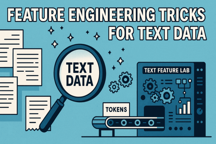
Image by Editor
Introduction
An increasing number of AI and machine learning-based systems feed on text data — language models are a notable example today. However, it is essential to note that machines do not truly understand language but rather numbers. Put another way: some feature engineering steps are typically needed to turn raw text data into useful numeric data features that these systems can digest and perform inference upon.
This article presents seven easy-to-implement tricks for performing feature engineering on text data. Depending on the complexity and requirements of the specific model to feed your data to, you may require a more or less ambitious set of these tricks.
- Numbers 1 to 5 are typically used for classical machine learning dealing with text, including decision-tree-based models, for instance.
- Numbers 6 and 7 are indispensable for deep learning models like recurrent neural networks and transformers, although number 2 (stemming and lemmatization) might still be necessary to enhance these models’ performance.
1. Removing Stopwords
Stopword removal helps reduce dimensionality: something indispensable for certain models that may suffer the so-called curse of dimensionality. Common words that may predominantly add noise to your data, like articles, prepositions, and auxiliary verbs, are removed, thereby keeping only those that convey most of the semantics in the source text.
Here’s how to do it in just a few lines of code (you may simply replace words with a list of text chunked into words of your own). We’ll use NLTK for the English stopword list:
|
import nltk nltk.download(‘stopwords’)
from nltk.corpus import stopwords words = [“this”,“is”,“a”,“crane”, “with”, “black”, “feathers”, “on”, “its”, “head”] stop_set = set(stopwords.words(‘english’)) filtered = [w for w in words if w.lower() not in stop_set] print(filtered) |
2. Stemming and Lemmatization
Reducing words to their root form can help merge variants (e.g., different tenses of a verb) into a unified feature. In deep learning models based on text embeddings, morphological aspects are usually captured, hence this step is rarely needed. However, when available data is very limited, it can still be useful because it alleviates sparsity and pushes the model to focus on core word meanings rather than assimilating redundant representations.
|
from nltk.stem import PorterStemmer stemmer = PorterStemmer() print(stemmer.stem(“running”)) |
3. Count-based Vectors: Bag of Words
One of the simplest approaches to turn text into numerical features in classical machine learning is the Bag of Words approach. It simply encodes word frequency into vectors. The result is a two-dimensional array of word counts describing simple baseline features: something advantageous for capturing the overall presence and relevance of words across documents, but limited because it fails to capture important aspects for understanding language like word order, context, or semantic relationships.
Still, it might end up being a simple yet effective approach for not-too-complex text classification models, for instance. Using scikit-learn:
|
from sklearn.feature_extraction.text import CountVectorizer cv = CountVectorizer() print(cv.fit_transform([“dog bites man”, “man bites dog”, “crane astonishes man”]).toarray()) |
4. TF-IDF Feature Extraction
Term Frequency — Inverse Document Frequency (TF-IDF) has long been one of natural language processing’s cornerstone approaches. It goes a step beyond Bag of Words and accounts for the frequency of words and their overall relevance not only at the single text (document) level, but at the dataset level. For example, in a text dataset containing 200 pieces of text or documents, words that appear frequently in a specific, narrow subset of texts but overall appear in few texts out of the existing 200 are deemed highly relevant: this is the idea behind inverse frequency. As a result, unique and important words are given higher weight.
By applying it to the following small dataset containing three texts, each word in each text is assigned a TF-IDF importance weight between 0 and 1:
|
from sklearn.feature_extraction.text import TfidfVectorizer tfidf = TfidfVectorizer() print(tfidf.fit_transform([“dog bites man”, “man bites dog”, “crane astonishes man”]).toarray()) |
5. Sentence-based N-Grams
Sentence-based n-grams help capture the interaction between words, for instance, “new” and “york.” Using the CountVectorizer class from scikit-learn, we can capture phrase-level semantics by setting the ngram_range parameter to incorporate sequences of multiple words. For instance, setting it to (1,2) creates features that are associated with both single words (unigrams) and combinations of two consecutive words (bigrams).
|
from sklearn.feature_extraction.text import CountVectorizer cv = CountVectorizer(ngram_range=(1,2)) print(cv.fit_transform([“new york is big”, “tokyo is even bigger”]).toarray()) |
6. Cleaning and Tokenization
Although there exist plenty of specialized tokenization algorithms out there in Python libraries like Transformers, the basic approach they are based on consists of removing punctuation, casing, and other symbols that downstream models may not understand. A simple cleaning and tokenization pipeline could consist of splitting text into words, lower-casing, and removing punctuation signs or other special characters. The result is a list of clean, normalized word units or tokens.
The re library for handling regular expressions can be used to build a simple tokenizer like this:
|
import re text = “Hello, World!!!” tokens = re.findall(r‘\b\w+\b’, text.lower()) print(tokens) |
7. Dense Features: Word Embeddings
Finally, one of the highlights and most powerful approaches to turn text into machine-readable information nowadays: word embeddings. They are great at capturing semantics, such as words with similar meaning, like ‘shogun’ and ‘samurai’, or ‘aikido’ and ‘jiujitsu’, which are encoded as numerically similar vectors (embeddings). In essence, words are mapped into a vector space using pre-defined approaches like Word2Vec or spaCy:
|
import spacy # Use a spaCy model with vectors (e.g., “en_core_web_md”) nlp = spacy.load(“en_core_web_md”) vec = nlp(“dog”).vector print(vec[:5]) # we only print a few dimensions of the dense embedding vector |
The output dimensionality of the embedding vector each word is transformed into is determined by the specific embedding algorithm and model used.
Wrapping Up
This article showcased seven useful tricks to make sense of raw text data when using it for machine learning and deep learning models that perform natural language processing tasks, such as text classification and summarization.


