
ROC AUC vs Precision-Recall for Imbalanced Data
Image by Editor | ChatGPT
Introduction
When building machine learning models to classify imbalanced data — i.e. datasets where the presence of one class (like spam email for example) is much less frequent than the presence of the other class (non-spam email, for instance) — certain traditional metrics like accuracy or even the ROC AUC (Receiving Operating Characteristic curve and the area under it) may not reflect the model performance in realistic terms, giving overly optimistic estimates due to the dominance of the so-called negative class.
Precision-recall curves (or PR curves for short), on the other hand, are designed to focus specifically on the positive, typically rarer class, which is a much more informative measure for skewed datasets due to class imbalance.
Through a discussion and three practical example scenarios, this article provides a comparison between ROC AUC and PR AUC — the area under both curves, taking values between 0 and 1 — across three imbalanced datasets, by training and evaluating a simple classifier based on logistic regression.
ROC AUC vs Precision-Recall
The ROC curve is the go-to approach to evaluate a classifier’s ability to discriminate between classes, namely by plotting the TPR (True Positive Rate, also called recall) against the FPR (False Positive Rate) for different thresholds for the probability of belonging to the positive class. Meanwhile, the precision-recall (PR) curve plots precision against recall for different thresholds, focusing on analyzing performance for positive class predictions. Therefore, it is particularly useful and informative for comprehensively evaluating classifiers trained on imbalanced datasets. The ROC curve, on the other hand, is less sensitive to class imbalance, being more suitable for evaluating classifiers built on rather balanced datasets, as well as in scenarios where the real-world cost of false positive and false negative predictions is similar.
In sum, back to the PR curve and class imbalance datasets, in high-stakes scenarios where correctly identifying positive-class instances is crucial (e.g. identifying the presence of a disease in a patient), the PR curve is a more reliable measure of the classifier’s performance.
On a more visual note, if we plot both curves alongside each other, we should get an increasing curve in the case of ROC and a decreasing curve in the case of PR. The closer the ROC curve gets to the (0,1) point, meaning the highest TPR and the lowest FPR, the better; whereas the closer the PR curve gets to the (1,1) point, meaning both precision and recall are at their maximum, the better. In both bases, getting closer to these “perfect model points” means the area under the curve or AUC becomes maximum: this is the numerical value we will seek in the examples that follow.
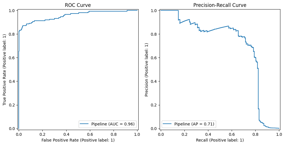
An example ROC curve and precision-recall curve
Image by Author
To illustrate the use and comparison between ROC AUC and precision-recall (PR curve for short), we will consider three datasets with different levels of class imbalance: from mildly to highly imbalanced. First, we will import everything we need for all three examples:
|
import pandas as pd from sklearn.datasets import load_breast_cancer from sklearn.model_selection import train_test_split from sklearn.linear_model import LogisticRegression from sklearn.preprocessing import StandardScaler from sklearn.pipeline import make_pipeline from sklearn.metrics import roc_auc_score, average_precision_score |
Example 1: Mild Imbalance and Different Performance Among Curves
The Pima Indians Diabetes Dataset is slightly imbalanced: about 35% of patients are diagnosed with diabetes (class label equals 1), and the other 65% have a negative diabetes diagnosis (class label equals 0).
This code loads the data, prepares it, trains a binary classifier based on logistic regression, and calculates the area under the two types of curves being discussed:
|
1 2 3 4 5 6 7 8 9 10 11 12 13 14 15 16 17 18 19 20 21 |
# Get the data cols = [“preg”,“glucose”,“bp”,“skin”,“insulin”,“bmi”,“pedigree”,“age”,“class”] df = pd.read_csv(“https://raw.githubusercontent.com/jbrownlee/Datasets/master/pima-indians-diabetes.data.csv”, names=cols)
# Separate labels and split into training-test X, y = df.drop(“class”, axis=1), df[“class”] X_train, X_test, y_train, y_test = train_test_split( X, y, stratify=y, test_size=0.3, random_state=42 )
# Scale data and train classifier clf = make_pipeline( StandardScaler(), LogisticRegression(max_iter=1000) ).fit(X_train, y_train)
# Obtain ROC AUC and precision-recall AUC probs = clf.predict_proba(X_test)[:,1] print(“ROC AUC:”, roc_auc_score(y_test, probs)) print(“PR AUC:”, average_precision_score(y_test, probs)) |
In this case, we got a ROC-AUC approximately equal to 0.838, and a PR-AUC of 0.733. As we can observe, the PR AUC (precision-recall) is moderately lower than the ROC AUC, which is a common pattern in many datasets because ROC AUC tends to overestimate classification performance on imbalanced datasets. The following example uses a similarly imbalanced dataset with different results.
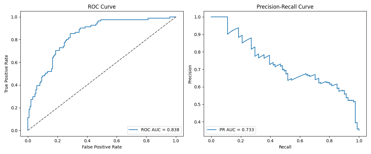
Image by Editor
Example 2: Mild Imbalance and Similar Performance Among Curves
Another imbalanced dataset with pretty similar class proportions to the previous ones is the Wisconsin Breast Cancer dataset available at scikit-learn, with 37% of instances being positive.
We apply a similar process to the previous example in the new dataset and analyze the results.
|
data = load_breast_cancer() X, y = data.data, (data.target==1).astype(int)
X_train, X_test, y_train, y_test = train_test_split( X, y, stratify=y, test_size=0.3, random_state=42 )
clf = make_pipeline( StandardScaler(), LogisticRegression(max_iter=1000) ).fit(X_train, y_train)
probs = clf.predict_proba(X_test)[:,1] print(“ROC AUC:”, roc_auc_score(y_test, probs)) print(“PR AUC:”, average_precision_score(y_test, probs)) |
In this case, we get an ROC AUC of 0.9981016355140186 and a PR AUC of 0.9988072626510498. This is an example that demonstrates that metric-specific model performance normally depends on a number of factors combined, and not only class imbalance. While class imbalance often may reflect a difference between PR vs ROC AUC, dataset characteristics like the size, complexity, signal strength from attributes, etc., are also influential. This particular dataset yielded a pretty well-performing classifier overall, which may partly explain its robustness to class imbalance (given the high PR AUC obtained).
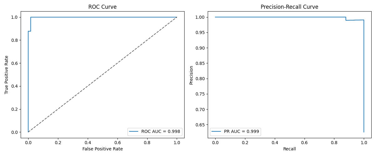
Image by Editor
Example 3: High Imbalance
The last example uses a highly imbalanced dataset, namely, the credit card fraud detection dataset, in which less than 1% of its nearly 285K instances belong to the positive class, indicating a transaction labeled as fraud.
|
1 2 3 4 5 6 7 8 9 10 11 12 13 14 15 16 17 |
url = ‘https://raw.githubusercontent.com/nsethi31/Kaggle-Data-Credit-Card-Fraud-Detection/master/creditcard.csv’ df = pd.read_csv(url)
X, y = df.drop(“Class”, axis=1), df[“Class”]
X_train, X_test, y_train, y_test = train_test_split( X, y, stratify=y, test_size=0.3, random_state=42 )
clf = make_pipeline( StandardScaler(), LogisticRegression(max_iter=2000) ).fit(X_train, y_train)
probs = clf.predict_proba(X_test)[:,1] print(“ROC AUC:”, roc_auc_score(y_test, probs)) print(“PR AUC:”, average_precision_score(y_test, probs)) |
This example clearly shows what typically occurs with highly imbalanced datasets: with an obtained ROC AUC of 0.957 and a PR AUC of 0.708, we have a strong overestimation of the model performance according to the ROC curve. This means that while ROC looks very promising, the reality is that positive cases are not being properly captured, due to being rare. A frequent pattern is that the stronger the imbalance, the bigger the difference between ROC AUC and PR AUC tends to be.
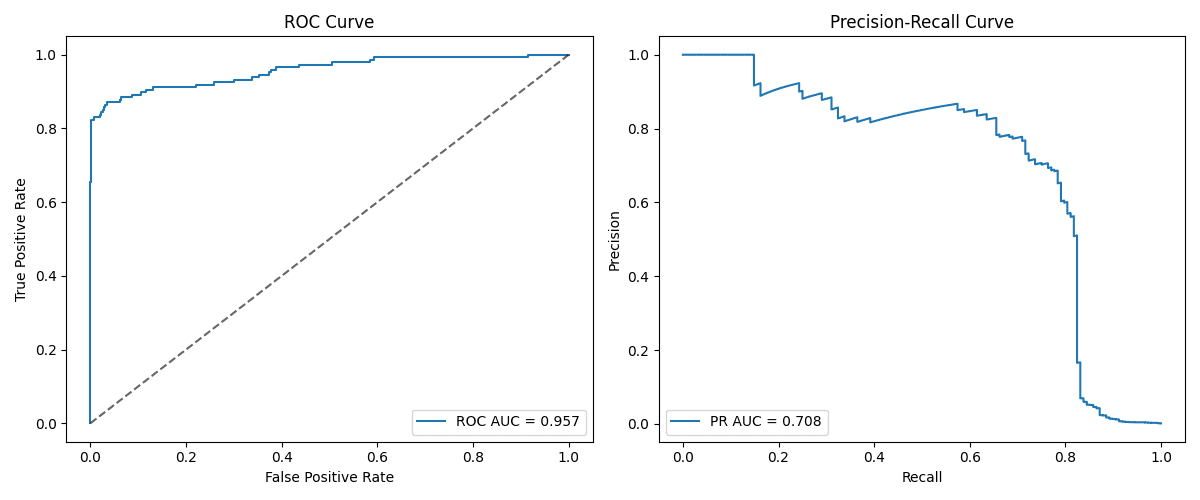
Image by Editor
Wrapping Up
This article discussed and compared two common metrics to evaluate classifier performance: ROC and precision-recall curves. Through three examples on imbalanced datasets, we showed the behavior and recommended uses of these metrics in different scenarios, with the general key lesson being that precision-recall curves tend to be a more informative and realistic way to evaluate classifiers for class-imbalanced data.
For further reading on how to navigate imbalanced datasets for classification, check out this article.