
Seeing Images Through the Eyes of Decision Trees
Image by Editor | ChatGPT
In this article, you’ll learn to:
- Turn unstructured, raw image data into structured, informative features.
- Train a decision tree classifier for image classification based on extracted image features.
- Apply the above concepts to the CIFAR-10 dataset for image classification.
Introduction
It’s no secret that decision tree-based models excel in a wide range of classification and regression tasks, often based on structured, tabular data. However, when used in combination with the right tools, decision trees can also be a powerful predictive tool for unstructured data such as text or images, and even for time series data.
This article demonstrates how decision trees can make sense of image data that has been converted into structured, meaningful features. More specifically, we will show how to turn raw, pixel-level image data into higher-level features that describe image properties like color histograms and edge counts. We’ll then leverage this information to perform predictive tasks, like classification, by training decision trees — all with the aid of Python’s scikit-learn library.
Think about it: it’ll be like making a decision tree’s behavior more like to how our human eyes work.
Building Decision Trees for Image Classification upon Image Features
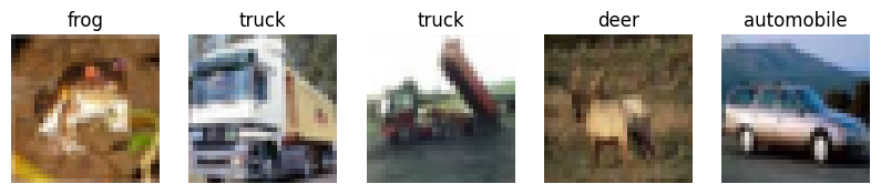
The CIFAR-10 dataset we will use for the tutorial is a collection of low-resolution, 32×32 pixel color images, with each pixel being described by three RGB values that define its color.
Although other commonly used models for image classification, like neural networks, can process images as grids of pixels, decision trees are designed to work with structured data; hence, our primary goal is to convert our raw image data into this structured format.
We start by loading the dataset, freely available in the TensorFlow library:
|
1 2 3 4 5 6 7 8 9 10 11 12 13 14 15 16 17 18 19 20 21 |
from tensorflow.keras.datasets import cifar10 import numpy as np import matplotlib.pyplot as plt
(X_train, y_train), (X_test, y_test) = cifar10.load_data() y_train = y_train.flatten() y_test = y_test.flatten()
class_names = [‘airplane’,‘automobile’,‘bird’,‘cat’,‘deer’, ‘dog’,‘frog’,‘horse’,‘ship’,‘truck’]
print(“Training set:”, X_train.shape, y_train.shape) print(“Test set:”, X_test.shape, y_test.shape)
# Optional: show a few samples (see article image above) fig, axes = plt.subplots(1, 5, figsize=(10, 3)) for i, ax in enumerate(axes): ax.imshow(X_train[i]) ax.set_title(class_names[y_train[i]]) ax.axis(‘off’) plt.show() |
Notice that the loaded dataset is already partitioned into training and test sets, and the output labels (10 different classes) are also separated from the input image data. We just need to allocate these elements correctly using Python tuples, as shown above. For clarity, we also store the class names in a Python list.
Next, we define the core function in our code. This function, called extract_features(), takes an image as input and extracts the desired image features. In our example, we will extract features associated with two main image properties: color histograms for each of the three RGB channels (red, green, and blue), and a measure of edge strength.
|
1 2 3 4 5 6 7 8 9 10 11 12 13 14 15 16 17 18 19 20 21 |
from skimage.color import rgb2gray from skimage.filters import sobel
def extract_features(images, bins_per_channel=8): features = [] for img in images: # Color histogram for each of the 3 RGB channels hist_features = [] for c in range(3): hist, _ = np.histogram(img[:,:,c], bins=bins_per_channel, range=(0, 255)) hist_features.extend(hist)
# Edge detection on grayscale image gray_img = rgb2gray(img) edges = sobel(gray_img) edge_strength = np.sum(edges > 0.1)
# Merging features features.append(hist_features + [edge_strength])
return np.array(features, dtype=np.float32) |
The number of bins for each computed color histogram is set to 8, so that the density of information describing the image color properties remains at a reasonable level. For edge detection, we use two functions from skimage: rgb2gray and sobel, which together help detect edges on grayscale versions of our original image.
Both subsets of features are put together, and the process repeats for every image in the dataset.
We now call the function twice: once for the training set, and once for the test set.
|
X_train_feats = extract_features(X_train) X_test_feats = extract_features(X_test)
print(“Feature vector size:”, X_train_feats.shape[1]) |
The resulting number of features containing information about RGB channel histograms and detected edges amounts to 25.
That was the hard part! Now we are largely ready to train a decision tree-based classifier that takes extracted features instead of raw image data as inputs. If you are already familiar with training scikit-learn models, the whole process is self-explanatory: we just need to make sure we pass the extracted features, rather than the raw images, as the training and evaluation inputs.
|
from sklearn.tree import DecisionTreeClassifier from sklearn.metrics import classification_report, accuracy_score
dt_model = DecisionTreeClassifier(random_state=42, max_depth=20) dt_model.fit(X_train_feats, y_train)
y_pred_dt = dt_model.predict(X_test_feats)
print(“MODEL 1. Decision Tree (Color histograms + Edge count):”) print(“Accuracy:”, accuracy_score(y_test, y_pred_dt)) print(classification_report(y_test, y_pred_dt, target_names=class_names)) |
Results:
|
1 2 3 4 5 6 7 8 9 10 11 12 13 14 15 16 17 |
Accuracy: 0.2594 precision recall f1–score support
airplane 0.33 0.33 0.33 1000 automobile 0.30 0.32 0.31 1000 bird 0.23 0.24 0.24 1000 cat 0.17 0.18 0.17 1000 deer 0.24 0.21 0.23 1000 dog 0.18 0.19 0.19 1000 frog 0.31 0.31 0.31 1000 horse 0.22 0.20 0.21 1000 ship 0.35 0.32 0.33 1000 truck 0.28 0.30 0.29 1000
accuracy 0.26 10000 macro avg 0.26 0.26 0.26 10000 weighted avg 0.26 0.26 0.26 10000 |
Unfortunately, the decision tree performs rather poorly on the extracted image features. And guess what: this is entirely normal and expected.
Reducing a 32×32 color image to just 25 explanatory features is an over-simplification that misses fine-grained cues and deeper details in the image that help discriminate, for instance, a bird from an airplane, or a dog from a cat. Keep in mind that image subsets belonging to the same class (e.g. ‘plane’) also have great intra-class variations in properties like color distribution. But the important take-home message here is to learn the how-to and limitations of image feature extraction for decision tree classifiers; achieving high accuracy is not our main goal in this tutorial!
Nonetheless, would things be any better if we trained a more advanced tree-based model, like a random forest classifier? Let’s find out:
|
from sklearn.ensemble import RandomForestClassifier
rf_model = RandomForestClassifier(n_estimators=100, random_state=42, n_jobs=–1) rf_model.fit(X_train_feats, y_train)
y_pred_rf = rf_model.predict(X_test_feats)
print(“MODEL 2. Random Forest (Color histograms + Edge count)”) print(“Accuracy:”, accuracy_score(y_test, y_pred_rf)) print(classification_report(y_test, y_pred_rf, target_names=class_names)) |
|
1 2 3 4 5 6 7 8 9 10 11 12 13 14 15 16 17 18 |
MODEL 2. Random Forest (Color histograms + Edge count) Accuracy: 0.3952 precision recall f1–score support
airplane 0.49 0.52 0.51 1000 automobile 0.37 0.48 0.42 1000 bird 0.36 0.30 0.33 1000 cat 0.27 0.19 0.22 1000 deer 0.38 0.34 0.36 1000 dog 0.32 0.29 0.30 1000 frog 0.45 0.50 0.47 1000 horse 0.39 0.35 0.36 1000 ship 0.46 0.53 0.49 1000 truck 0.41 0.47 0.44 1000
accuracy 0.40 10000 macro avg 0.39 0.40 0.39 10000 weighted avg 0.39 0.40 0.39 10000 |
Slight improvement here, but still far from perfect. Eager for some homework? Try applying what we learned in this article to an even simpler dataset, like MNIST or fashion MNIST, and see how it performs. It only got a pass mark for classifying airplanes, still failing for the other nine classes!
A Last Try: Adding Deeper Features with HOG
If the information level of the features extracted before was arguably too shallow, how about adding more features that capture more nuanced aspects of the image? One could be HOG (Histogram of Oriented Gradients), which can capture properties like shape and texture, adding a significant number of extra features.
The following code expands the feature extraction process and applies it to train another random forest classifier (fingers crossed).
|
1 2 3 4 5 6 7 8 9 10 11 12 13 14 15 16 17 18 19 20 21 22 23 24 25 26 27 28 29 30 31 32 33 34 35 |
from skimage.color import rgb2gray from skimage.feature import hog from skimage.filters import sobel import numpy as np
def extract_rich_features(images, bins_per_channel=16, hog_pixels_per_cell=(8,8)): features = [] for img in images: hist_features = [] for c in range(3): # R, G, B hist, _ = np.histogram(img[:,:,c], bins=bins_per_channel, range=(0, 255)) hist_features.extend(hist)
gray_img = rgb2gray(img) hog_features = hog( gray_img, pixels_per_cell=hog_pixels_per_cell, cells_per_block=(1,1), orientations=9, block_norm=‘L2-Hys’, feature_vector=True )
edges = sobel(gray_img) edge_density = np.sum(edges > 0.1) / edges.size
combined = np.hstack([hist_features, hog_features, edge_density]) features.append(combined)
return np.array(features, dtype=np.float32)
X_train_feats = extract_rich_features(X_train) X_test_feats = extract_rich_features(X_test)
print(“New feature vector size:”, X_train_feats.shape[1]) |
Training a new classifier (we now have 193 features instead of 25!):
|
from sklearn.ensemble import RandomForestClassifier from sklearn.metrics import classification_report, accuracy_score
rf_model = RandomForestClassifier(n_estimators=100, random_state=42, n_jobs=–1) rf_model.fit(X_train_feats, y_train)
y_pred_rf = rf_model.predict(X_test_feats)
print(“MODEL 3. Random Forest (Color histograms + HOG + Edge density)”) print(“Accuracy:”, accuracy_score(y_test, y_pred_rf)) print(classification_report(y_test, y_pred_rf, target_names=class_names)) |
Results:
|
1 2 3 4 5 6 7 8 9 10 11 12 13 14 15 16 17 18 |
MODEL 3. Random Forest (Color histograms + HOG + Edge density) Accuracy: 0.486 precision recall f1–score support
airplane 0.57 0.62 0.59 1000 automobile 0.56 0.67 0.61 1000 bird 0.45 0.32 0.37 1000 cat 0.34 0.25 0.29 1000 deer 0.43 0.43 0.43 1000 dog 0.39 0.42 0.40 1000 frog 0.52 0.56 0.54 1000 horse 0.49 0.44 0.46_ 1000 ship 0.54 0.59 0.56 1000 truck 0.49 0.58 0.53 1000
accuracy 0.49 10000 macro avg 0.48 0.49 0.48 10000 weighted avg 0.48 0.49 0.48 10000 |
Well, slow but steady, we managed to get a humble improvement, at least now several classes get a pass mark in some of the evaluation metrics, not just ‘airplane’. But still a long way to go: lesson learned.
Wrapping Up
This article showed how to train decision tree models capable of dealing with visual features extracted from image data, like color channel distributions and detected edges, highlighting both the capabilities and limitations of this approach.